Linear models

A simple linear model

Example dataset: forest trees

• Download this dataset

download.file("https://raw.githubusercontent.com/Pakillo/LM-GLM-GLMM-intro/trees/data/trees.csv",
              destfile = "trees.csv", mode = "wb")

• Import:

trees <- read.csv("trees.csv")
head(trees)

  site   dbh height    sex dead
1    4 29.68   36.1   male    0
2    5 33.29   42.3   male    0
3    2 28.03   41.9 female    0
4    5 39.86   46.5 female    0
5    1 47.94   43.9 female    0
6    1 10.82   26.2   male    0

Questions

• What is the relationship between DBH and height?

• Do taller trees have bigger trunks?

• Can we predict height from DBH? How well?

Plot your data first!

Exploratory Data Analysis (EDA)

Outliers

plot(trees$height)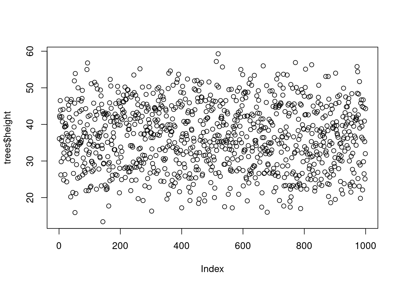

Histogram of response variable

hist(trees$height)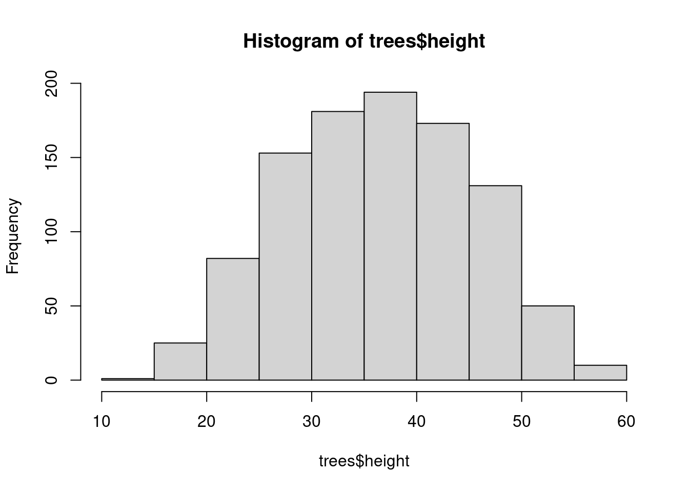

Histogram of predictor variable

hist(trees$dbh)

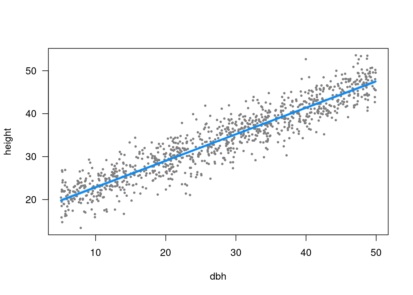
Scatterplot

plot(height ~ dbh, data = trees, las = 1)

Model fitting

Now fit model

Hint: lm

m1 <- lm(height ~ dbh, data = trees)

which corresponds to

\[ \begin{aligned} Height_{i} = a + b \cdot DBH_{i} + \varepsilon _{i} \\ \varepsilon _{i}\sim N\left( 0,\sigma^2 \right) \\ \end{aligned} \]

Package equatiomatic returns model structure

library("equatiomatic")
m1 <- lm(height ~ dbh, data = trees)
equatiomatic::extract_eq(m1)

equatiomatic::extract_eq(m1, use_coefs = TRUE)

Model interpretation

What does this mean?

summary(m1)

Call:
lm(formula = height ~ dbh, data = trees)

Residuals:
     Min       1Q   Median       3Q      Max 
-13.3270  -2.8978   0.1057   2.7924  12.9511 

Coefficients:
            Estimate Std. Error t value Pr(>|t|)    
(Intercept) 19.33920    0.31064   62.26   <2e-16 ***
dbh          0.61570    0.01013   60.79   <2e-16 ***
---
Signif. codes:  0 '***' 0.001 '**' 0.01 '*' 0.05 '.' 0.1 ' ' 1

Residual standard error: 4.093 on 998 degrees of freedom
Multiple R-squared:  0.7874,    Adjusted R-squared:  0.7871 
F-statistic:  3695 on 1 and 998 DF,  p-value: < 2.2e-16

Estimated distribution of the intercept parameter

library("easystats")

# Attaching packages: easystats 0.7.0
✔ bayestestR  0.13.1   ✔ correlation 0.8.4 
✔ datawizard  0.9.0    ✔ effectsize  0.8.6 
✔ insight     0.19.6   ✔ modelbased  0.8.6 
✔ performance 0.10.8   ✔ parameters  0.21.3
✔ report      0.5.7    ✔ see         0.8.1 

parameters(m1)[1,]

Parameter   | Coefficient |   SE |         95% CI | t(998) |      p
-------------------------------------------------------------------
(Intercept) |       19.34 | 0.31 | [18.73, 19.95] |  62.26 | < .001

Uncertainty intervals (equal-tailed) and p-values (two-tailed) computed
  using a Wald t-distribution approximation.

plot(simulate_parameters(m1), show_intercept = TRUE)

Estimated distribution of the slope parameter

parameters::parameters(m1)[2,]

Parameter | Coefficient |   SE |       95% CI | t(998) |      p
---------------------------------------------------------------
dbh       |        0.62 | 0.01 | [0.60, 0.64] |  60.79 | < .001

Uncertainty intervals (equal-tailed) and p-values (two-tailed) computed
  using a Wald t-distribution approximation.

plot(simulate_parameters(m1))

Distribution of residuals

hist(residuals(m1))

Degrees of freedom

DF = n - p

n = sample size

p = number of estimated parameters

R-squared

Proportion of ‘explained’ variance

\(R^{2} = 1 - \frac{Residual Variation}{Total Variation}\)

Adjusted R-squared

Accounts for model complexity

(number of parameters)

\(R^2_{adj} = 1 - (1 - R^2) \frac{n - 1}{n - p - 1}\)

Quiz

https://pollev.com/franciscorod726

Retrieving model coefficients

coef(m1)

(Intercept)         dbh 
 19.3391968   0.6157036 

Confidence intervals for parameters

confint(m1)

                 2.5 %    97.5 %
(Intercept) 18.7296053 19.948788
dbh          0.5958282  0.635579

Retrieving model parameters (easystats)

parameters(m1)

Parameter   | Coefficient |   SE |         95% CI | t(998) |      p
-------------------------------------------------------------------
(Intercept) |       19.34 | 0.31 | [18.73, 19.95] |  62.26 | < .001
dbh         |        0.62 | 0.01 | [ 0.60,  0.64] |  60.79 | < .001

Uncertainty intervals (equal-tailed) and p-values (two-tailed) computed
  using a Wald t-distribution approximation.

https://easystats.github.io/parameters/

Communicating results

Avoid dichotomania of statistical significance

• “Never conclude there is ‘no difference’ or ‘no association’ just because p > 0.05 or CI includes zero”

• Estimate and communicate effect sizes and their uncertainty

• https://doi.org/10.1038/d41586-019-00857-9

Communicating results

• We found a significant relationship between DBH and Height (p<0.05).

• We found a {significant} positive relationship between DBH and Height {(p<0.05)} (b = 0.61, SE = 0.01).

• (add p-value if you wish)

Models that describe themselves (easystats)

report(m1)

We fitted a linear model (estimated using OLS) to predict height with dbh
(formula: height ~ dbh). The model explains a statistically significant and
substantial proportion of variance (R2 = 0.79, F(1, 998) = 3695.40, p < .001,
adj. R2 = 0.79). The model's intercept, corresponding to dbh = 0, is at 19.34
(95% CI [18.73, 19.95], t(998) = 62.26, p < .001). Within this model:

  - The effect of dbh is statistically significant and positive (beta = 0.62, 95%
CI [0.60, 0.64], t(998) = 60.79, p < .001; Std. beta = 0.89, 95% CI [0.86,
0.92])

Standardized parameters were obtained by fitting the model on a standardized
version of the dataset. 95% Confidence Intervals (CIs) and p-values were
computed using a Wald t-distribution approximation.

https://easystats.github.io/report/

Generating table with model results: modelsummary

library("modelsummary")

Attaching package: 'modelsummary'

The following object is masked from 'package:parameters':

    supported_models

The following object is masked from 'package:insight':

    supported_models

modelsummary(m1, output = "html")  ## Word, PDF, PowerPoint, png...

	(1)
(Intercept)	19.339
	(0.311)
dbh	0.616
	(0.010)
Num.Obs.	1000
R2	0.787
R2 Adj.	0.787
AIC	5660.3
BIC	5675.0
Log.Lik.	−2827.125
F	3695.395
RMSE	4.09

https://modelsummary.com/

Generating table with model results: modelsummary

modelsummary(m1, fmt = 2, 
             estimate = "{estimate} ({std.error})", 
             statistic = NULL,
             gof_map = c("nobs", "r.squared", "rmse"),
             output = "html")

	(1)
(Intercept)	19.34 (0.31)
dbh	0.62 (0.01)
Num.Obs.	1000
R2	0.787
RMSE	4.09

Visualising fitted model

Plot model: visreg

library("visreg")

visreg(m1)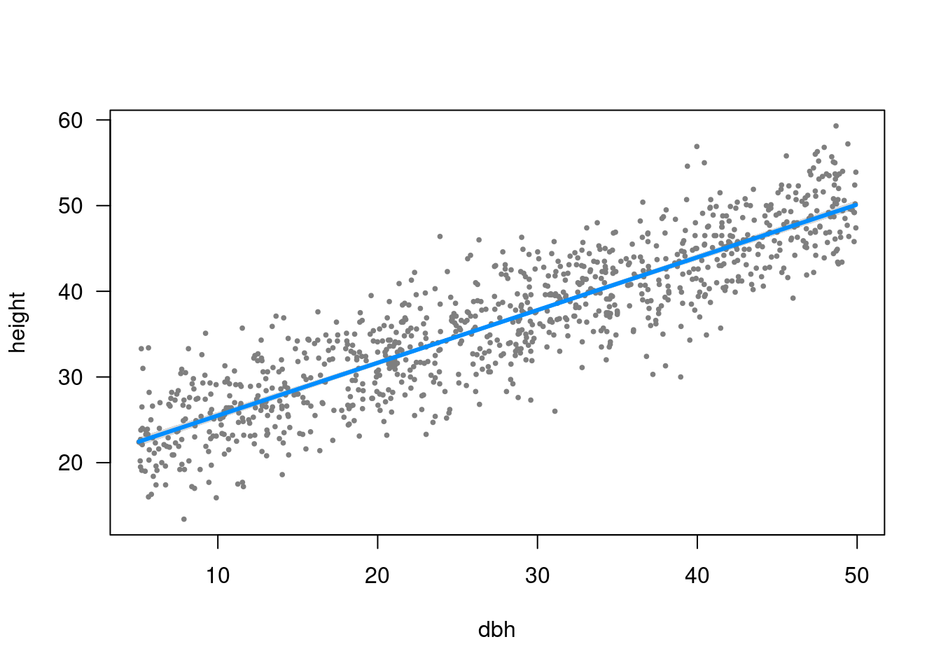

visreg can use ggplot2 too

visreg(m1, gg = TRUE) + theme_bw()

https://pbreheny.github.io/visreg

Plot (easystats)

plot(estimate_expectation(m1))

Plot (modelsummary)

modelplot(m1)

Plot model parameters with easystats (see package)

plot(parameters(m1), show_intercept = TRUE, show_labels = TRUE)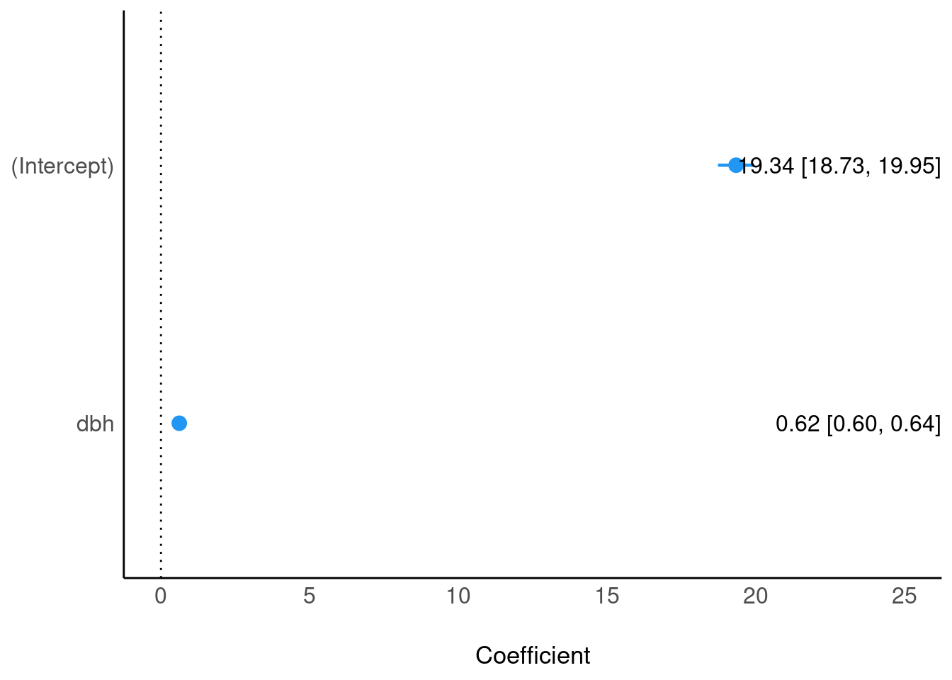

Plot parameters’ estimated distribution

plot(simulate_parameters(m1))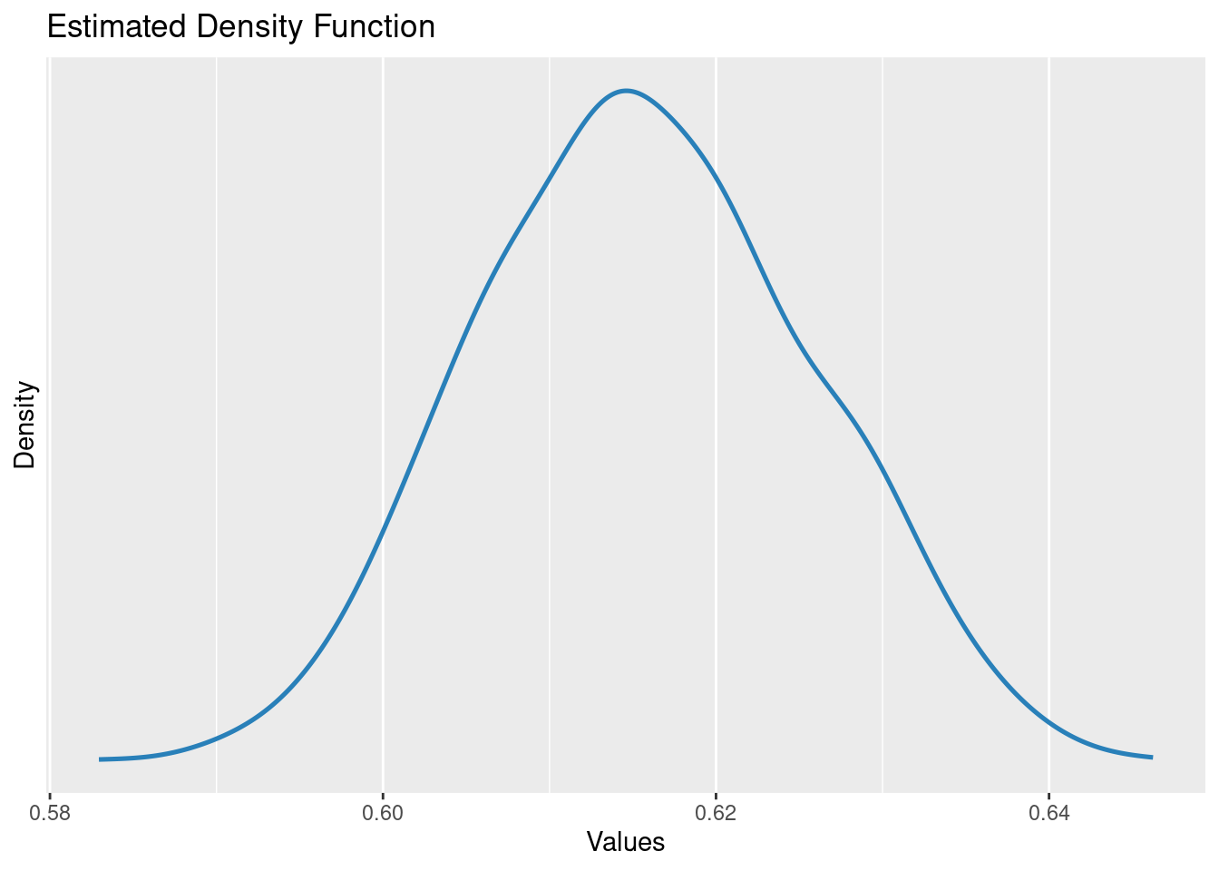

Model checking

Linear model assumptions

• Linearity (transformations, GAM…)

• Residuals:

  • Independent
  • Equal variance
  • Normal

• Negligible measurement error in predictors

Are residuals normal?

hist(residuals(m1))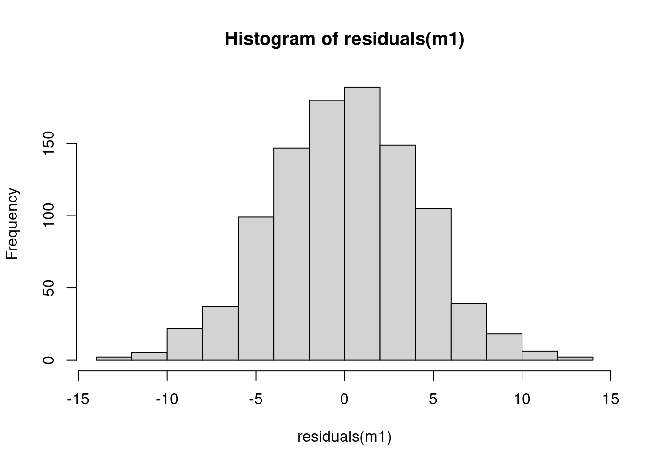

SD = 4.09

Model checking: plot(model)

def.par <- par(no.readonly = TRUE)
layout(matrix(1:4, nrow=2))
plot(m1)

par(def.par)

Model checking with performance (easystats)

check_model(m1)

https://easystats.github.io/performance/articles/check_model.html

A dashboard to explore the full model

model_dashboard(m1)

Making predictions with easystats

Estimate expected values

pred <- estimate_expectation(m1)
head(pred)

Model-based Expectation

dbh   | Predicted |   SE |         95% CI | Residuals
-----------------------------------------------------
29.68 |     37.61 | 0.13 | [37.36, 37.87] |     -1.51
33.29 |     39.84 | 0.14 | [39.56, 40.11] |      2.46
28.03 |     36.60 | 0.13 | [36.34, 36.85] |      5.30
39.86 |     43.88 | 0.18 | [43.53, 44.23] |      2.62
47.94 |     48.86 | 0.24 | [48.38, 49.33] |     -4.96
10.82 |     26.00 | 0.22 | [25.58, 26.42] |      0.20

Variable predicted: height

Expected values given DBH

plot(estimate_expectation(m1))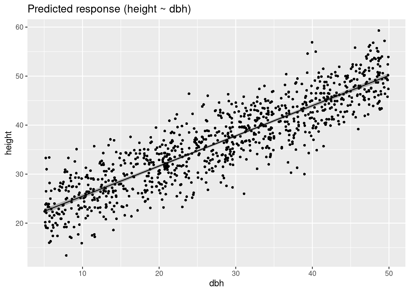

Calibration plot: observed vs predicted

pred$height.obs <- trees$height
plot(height.obs ~ Predicted, data = pred, xlim = c(15, 60), ylim = c(15, 60))
abline(a = 0, b = 1)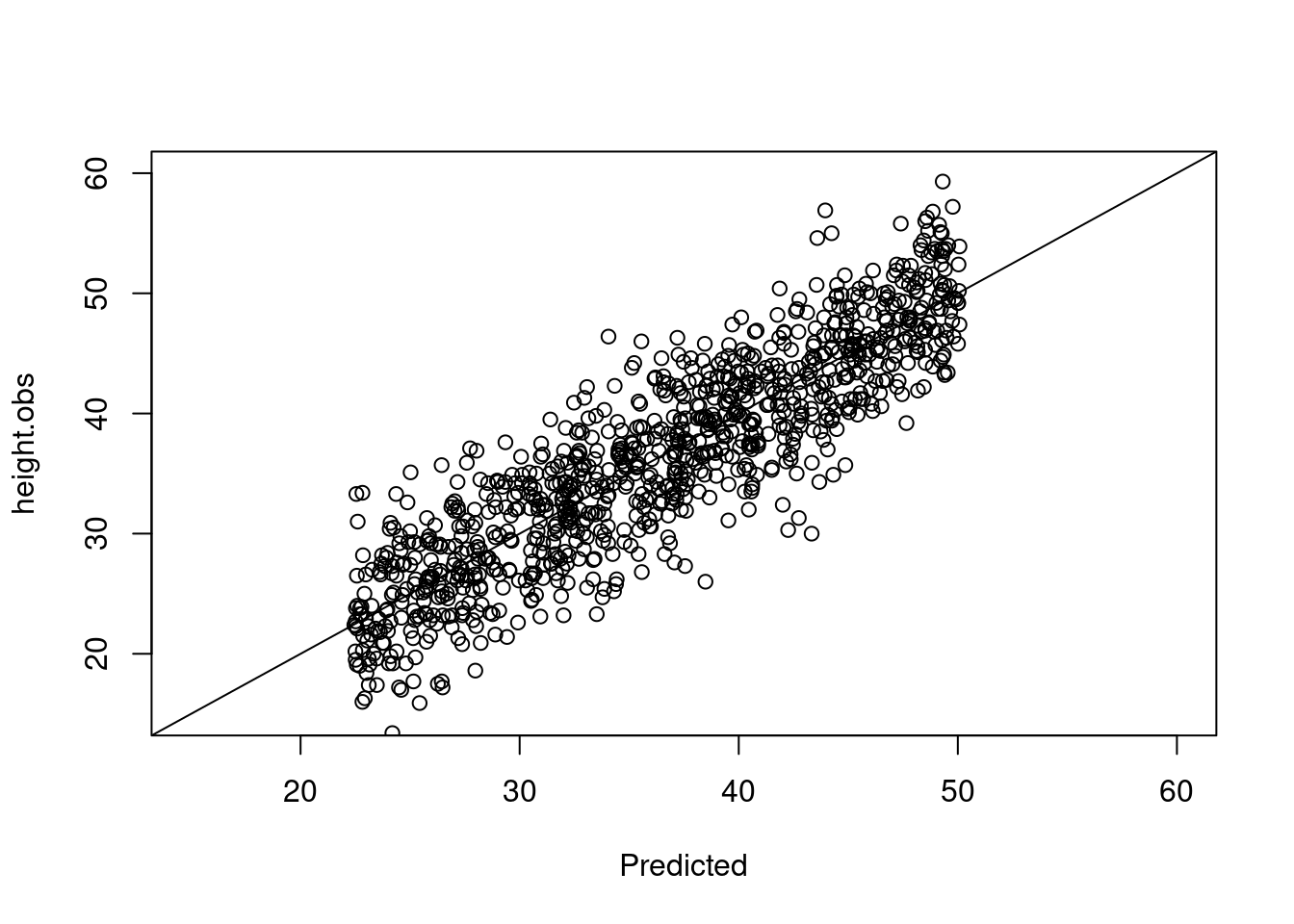

Estimate prediction interval

Accounting for residual variation!

pred <- estimate_prediction(m1)
head(pred)

Model-based Prediction

dbh   | Predicted |   SE |         95% CI | Residuals
-----------------------------------------------------
29.68 |     37.61 | 4.09 | [29.58, 45.65] |     -1.51
33.29 |     39.84 | 4.10 | [31.80, 47.87] |      2.46
28.03 |     36.60 | 4.09 | [28.56, 44.63] |      5.30
39.86 |     43.88 | 4.10 | [35.84, 51.92] |      2.62
47.94 |     48.86 | 4.10 | [40.81, 56.90] |     -4.96
10.82 |     26.00 | 4.10 | [17.96, 34.04] |      0.20

Variable predicted: height

Confidence vs Prediction interval

plot(estimate_expectation(m1))

plot(estimate_prediction(m1))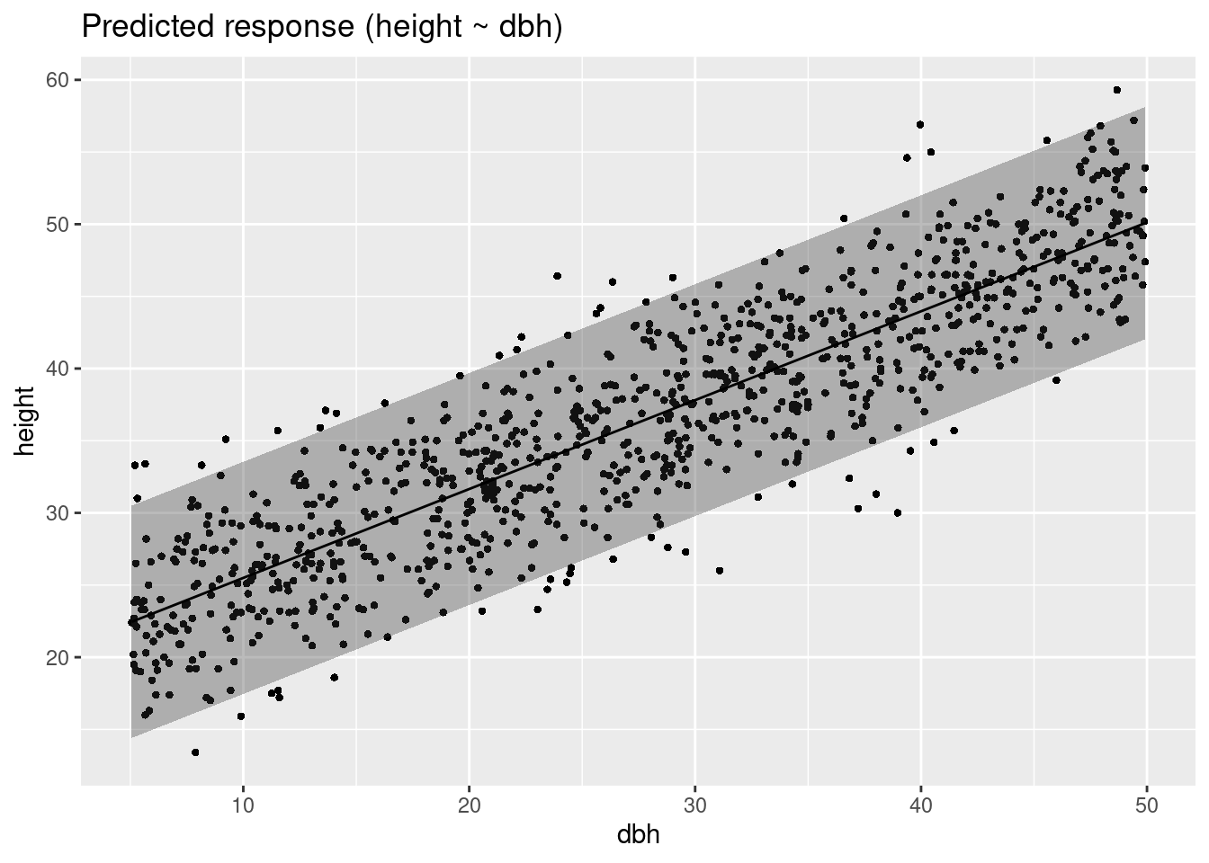

Make predictions for new data

estimate_expectation(m1, data = data.frame(dbh = 39))

Model-based Expectation

dbh   | Predicted |   SE |         95% CI
-----------------------------------------
39.00 |     43.35 | 0.17 | [43.01, 43.69]

Variable predicted: height

estimate_prediction(m1, data = data.frame(dbh = 39))

Model-based Prediction

dbh   | Predicted |   SE |         95% CI
-----------------------------------------
39.00 |     43.35 | 4.10 | [35.31, 51.39]

Variable predicted: height

Workflow

• Visualise data

• Understand fitted model (summary)

• Visualise model (visreg…)

• Check model (plot, check_model, calibration plot…)

• Predict (predict, estimate_expectation, estimate_prediction)

Categorical predictors (factors)

Q: Does tree height vary with sex?

boxplot(height ~ sex, data = trees)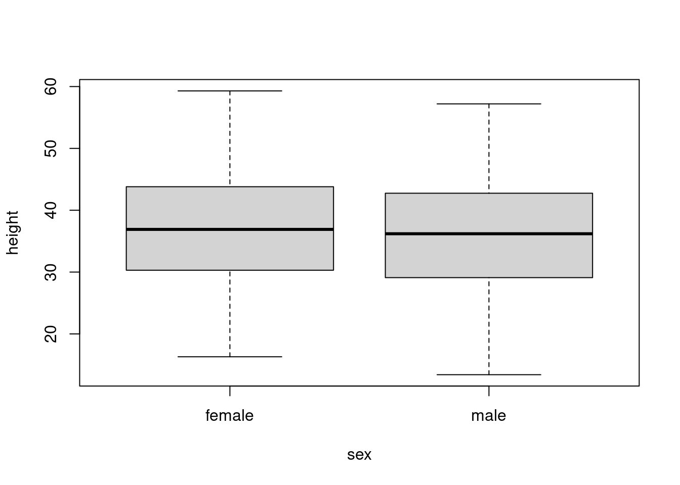

Model height ~ sex

m2 <- lm(height ~ sex, data = trees)
summary(m2)

Call:
lm(formula = height ~ sex, data = trees)

Residuals:
     Min       1Q   Median       3Q      Max 
-22.6881  -6.7881  -0.0097   6.7261  22.3687 

Coefficients:
            Estimate Std. Error t value Pr(>|t|)    
(Intercept)  36.9312     0.3981  92.778   <2e-16 ***
sexmale      -0.8432     0.5607  -1.504    0.133    
---
Signif. codes:  0 '***' 0.001 '**' 0.01 '*' 0.05 '.' 0.1 ' ' 1

Residual standard error: 8.865 on 998 degrees of freedom
Multiple R-squared:  0.002261,  Adjusted R-squared:  0.001261 
F-statistic: 2.261 on 1 and 998 DF,  p-value: 0.133

Linear model with categorical predictors

m2 <- lm(height ~ sex, data = trees)

corresponds to

\[ \begin{aligned} Height_{i} = a + b_{male} + \varepsilon _{i} \\ \varepsilon _{i}\sim N\left( 0,\sigma^2 \right) \\ \end{aligned} \]

Model height ~ sex

m2 <- lm(height ~ sex, data = trees)
summary(m2)

Call:
lm(formula = height ~ sex, data = trees)

Residuals:
     Min       1Q   Median       3Q      Max 
-22.6881  -6.7881  -0.0097   6.7261  22.3687 

Coefficients:
            Estimate Std. Error t value Pr(>|t|)    
(Intercept)  36.9312     0.3981  92.778   <2e-16 ***
sexmale      -0.8432     0.5607  -1.504    0.133    
---
Signif. codes:  0 '***' 0.001 '**' 0.01 '*' 0.05 '.' 0.1 ' ' 1

Residual standard error: 8.865 on 998 degrees of freedom
Multiple R-squared:  0.002261,  Adjusted R-squared:  0.001261 
F-statistic: 2.261 on 1 and 998 DF,  p-value: 0.133

Quiz

https://pollev.com/franciscorod726

Let’s read the model report…

report(m2)

We fitted a linear model (estimated using OLS) to predict height with sex
(formula: height ~ sex). The model explains a statistically not significant and
very weak proportion of variance (R2 = 2.26e-03, F(1, 998) = 2.26, p = 0.133,
adj. R2 = 1.26e-03). The model's intercept, corresponding to sex = female, is
at 36.93 (95% CI [36.15, 37.71], t(998) = 92.78, p < .001). Within this model:

  - The effect of sex [male] is statistically non-significant and negative (beta
= -0.84, 95% CI [-1.94, 0.26], t(998) = -1.50, p = 0.133; Std. beta = -0.10,
95% CI [-0.22, 0.03])

Standardized parameters were obtained by fitting the model on a standardized
version of the dataset. 95% Confidence Intervals (CIs) and p-values were
computed using a Wald t-distribution approximation.

Estimated distribution of the intercept parameter

Intercept = Height of females

parameters(m2)[1,]

Parameter   | Coefficient |   SE |         95% CI | t(998) |      p
-------------------------------------------------------------------
(Intercept) |       36.93 | 0.40 | [36.15, 37.71] |  92.78 | < .001

Uncertainty intervals (equal-tailed) and p-values (two-tailed) computed
  using a Wald t-distribution approximation.

plot(simulate_parameters(m2), show_intercept = TRUE)

Estimated distribution of the beta parameter

beta = height difference of males vs females

parameters(m2)[2,]

Parameter  | Coefficient |   SE |        95% CI | t(998) |     p
----------------------------------------------------------------
sex [male] |       -0.84 | 0.56 | [-1.94, 0.26] |  -1.50 | 0.133

Uncertainty intervals (equal-tailed) and p-values (two-tailed) computed
  using a Wald t-distribution approximation.

plot(simulate_parameters(m2))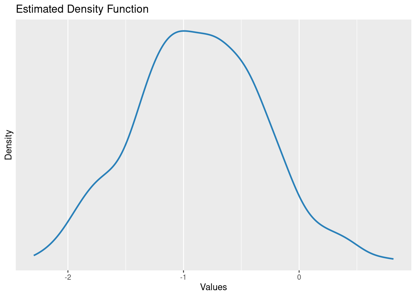

Analysing differences among factor levels

estimate_means(m2)

We selected `at = c("sex")`.

Estimated Marginal Means

sex    |  Mean |   SE |         95% CI
--------------------------------------
male   | 36.09 | 0.39 | [35.31, 36.86]
female | 36.93 | 0.40 | [36.15, 37.71]

Marginal means estimated at sex

estimate_contrasts(m2)

No variable was specified for contrast estimation. Selecting `contrast = "sex"`.

Marginal Contrasts Analysis

Level1 | Level2 | Difference |        95% CI |   SE | t(998) |     p
--------------------------------------------------------------------
male   | female |      -0.84 | [-1.94, 0.26] | 0.56 |  -1.50 | 0.133

Marginal contrasts estimated at sex
p-value adjustment method: Holm (1979)

Visualising the fitted model

Plot (visreg)

visreg(m2)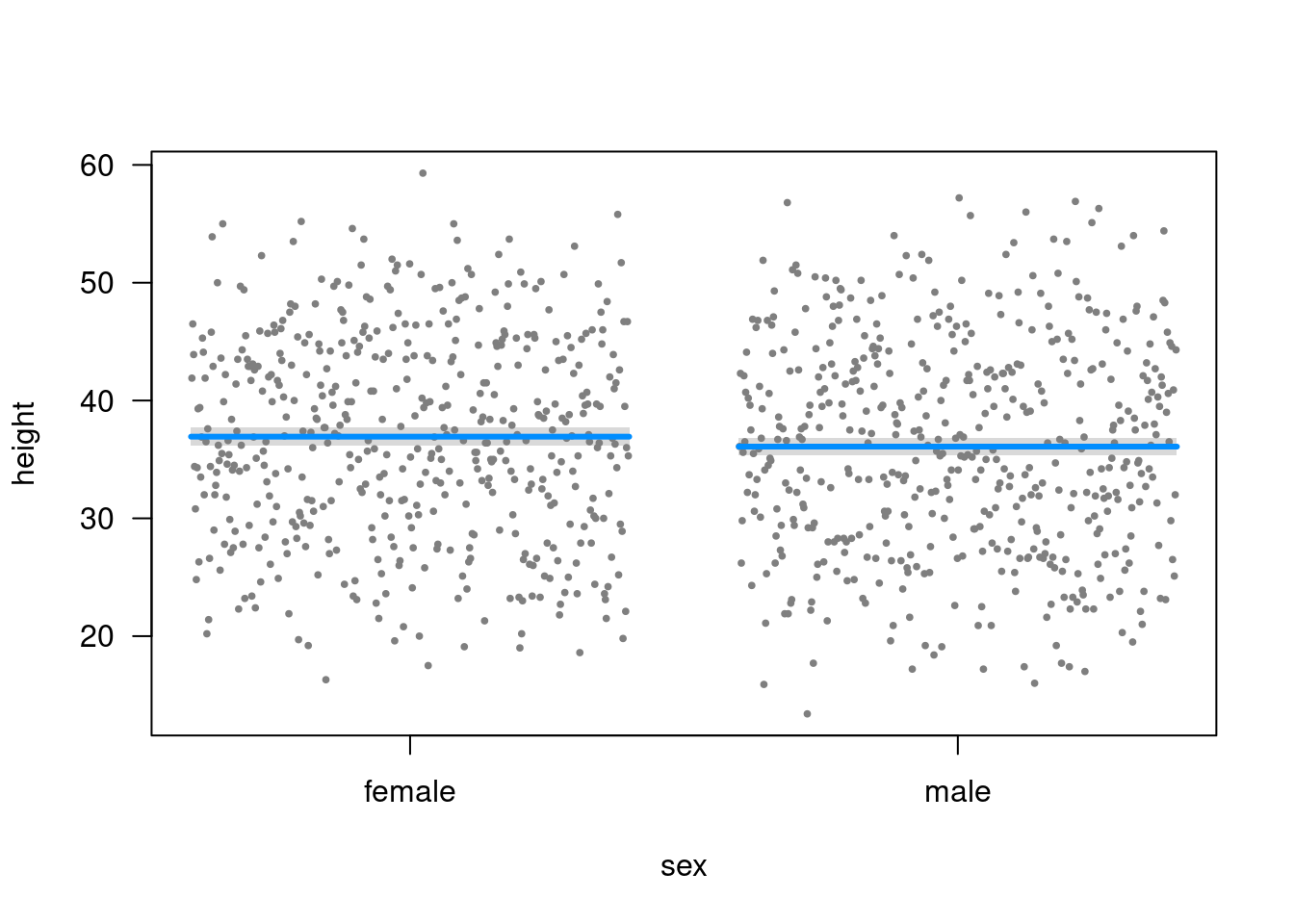

Plot (easystats)

plot(estimate_means(m2))

We selected `at = c("sex")`.

Model checking

Model checking: residuals

hist(resid(m2))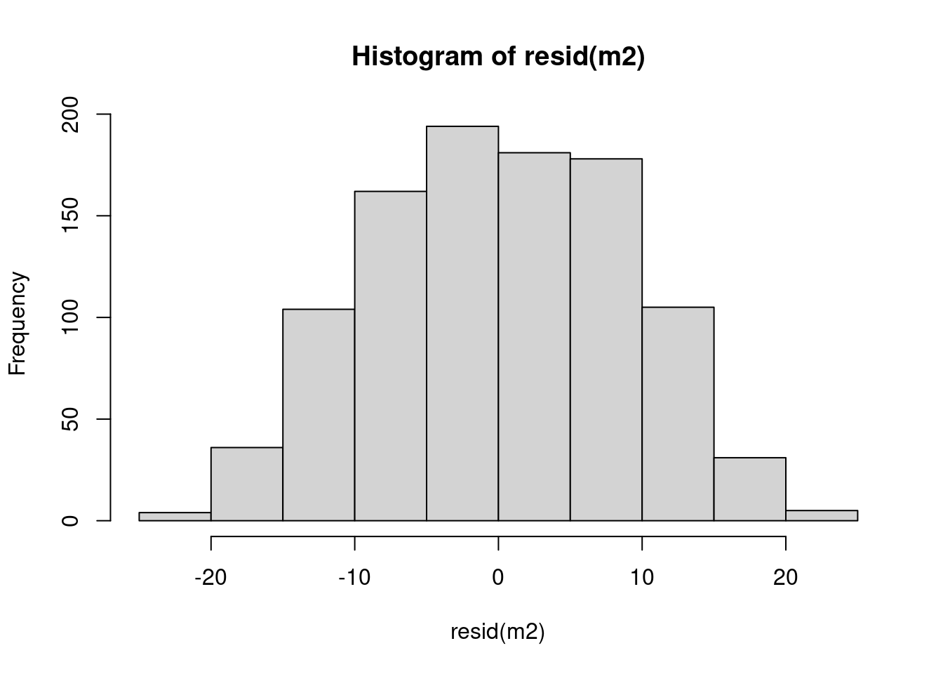

def.par <- par(no.readonly = TRUE)
layout(matrix(1:4, nrow=2))
plot(m2)

par(def.par)

Model checking (easystats)

check_model(m2)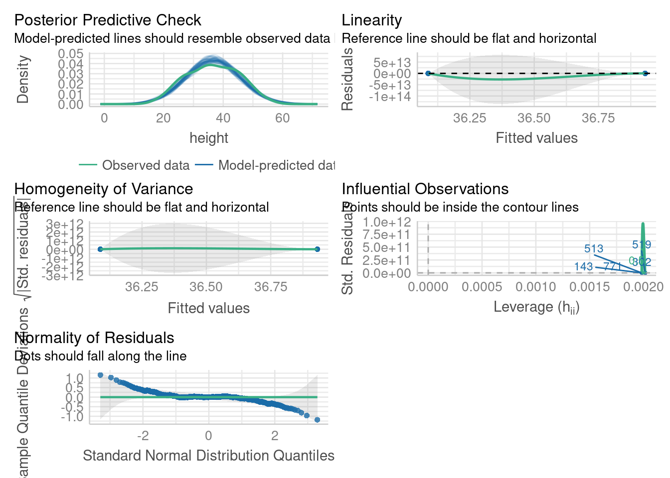

Q: Does height differ among field sites?

Quiz

https://pollev.com/franciscorod726

Plot data first

plot(height ~ site, data = trees)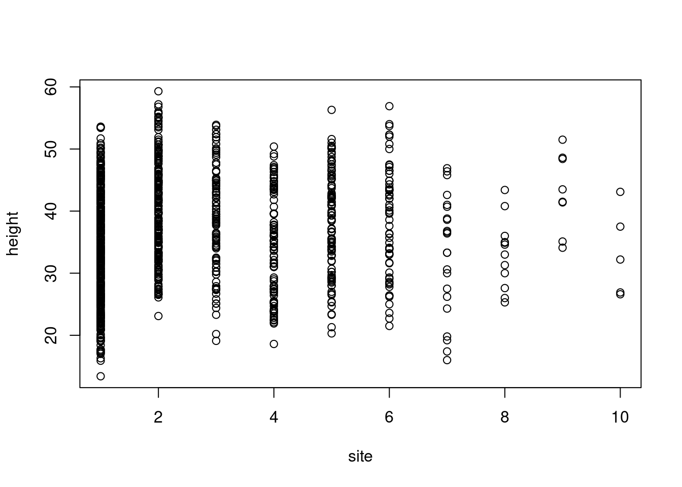

Linear model with categorical predictors

m3 <- lm(height ~ site, data = trees)

\[ \begin{aligned} y_{i} = a + b_{site2} + c_{site3} + d_{site4} + e_{site5} +...+ \varepsilon _{i} \\ \varepsilon _{i}\sim N\left( 0,\sigma^2 \right) \\ \end{aligned} \]

Model Height ~ site

All right here?

m3 <- lm(height ~ site, data = trees)
summary(m3)

Call:
lm(formula = height ~ site, data = trees)

Residuals:
     Min       1Q   Median       3Q      Max 
-22.4498  -6.7049   0.0709   6.7537  23.0640 

Coefficients:
            Estimate Std. Error t value Pr(>|t|)    
(Intercept)  35.4636     0.4730  74.975  < 2e-16 ***
site          0.3862     0.1413   2.733  0.00639 ** 
---
Signif. codes:  0 '***' 0.001 '**' 0.01 '*' 0.05 '.' 0.1 ' ' 1

Residual standard error: 8.842 on 998 degrees of freedom
Multiple R-squared:  0.007429,  Adjusted R-squared:  0.006435 
F-statistic:  7.47 on 1 and 998 DF,  p-value: 0.006385

site is a factor!

trees$site <- as.factor(trees$site)

Model Height ~ site

m3 <- lm(height ~ site, data = trees)
summary(m3)

Call:
lm(formula = height ~ site, data = trees)

Residuals:
     Min       1Q   Median       3Q      Max 
-20.4416  -6.9004   0.0379   6.3051  19.7584 

Coefficients:
            Estimate Std. Error t value Pr(>|t|)    
(Intercept)  33.8416     0.4266  79.329  < 2e-16 ***
site2         6.3411     0.7126   8.899  < 2e-16 ***
site3         4.9991     0.9828   5.086 4.36e-07 ***
site4         0.5329     0.9872   0.540  0.58949    
site5         4.3723     0.9425   4.639 3.97e-06 ***
site6         4.7601     1.1709   4.065 5.18e-05 ***
site7        -0.7416     1.8506  -0.401  0.68871    
site8        -0.6832     2.4753  -0.276  0.78258    
site9         9.1709     3.0165   3.040  0.00243 ** 
site10       -0.5816     3.8013  -0.153  0.87843    
---
Signif. codes:  0 '***' 0.001 '**' 0.01 '*' 0.05 '.' 0.1 ' ' 1

Residual standard error: 8.446 on 990 degrees of freedom
Multiple R-squared:  0.1016,    Adjusted R-squared:  0.09344 
F-statistic: 12.44 on 9 and 990 DF,  p-value: < 2.2e-16

Estimated parameter distributions

plot(simulate_parameters(m3))

Estimated tree heights for each site

estimate_means(m3)

We selected `at = c("site")`.

Estimated Marginal Means

site |  Mean |   SE |         95% CI
------------------------------------
1    | 33.84 | 0.43 | [33.00, 34.68]
2    | 40.18 | 0.57 | [39.06, 41.30]
3    | 38.84 | 0.89 | [37.10, 40.58]
4    | 34.37 | 0.89 | [32.63, 36.12]
5    | 38.21 | 0.84 | [36.56, 39.86]
6    | 38.60 | 1.09 | [36.46, 40.74]
7    | 33.10 | 1.80 | [29.57, 36.63]
8    | 33.16 | 2.44 | [28.37, 37.94]
9    | 43.01 | 2.99 | [37.15, 48.87]
10   | 33.26 | 3.78 | [25.85, 40.67]

Marginal means estimated at site

Plot estimated tree heights for each site

plot(estimate_means(m3))

We selected `at = c("site")`.

Analysing differences among factor levels

For finer control see emmeans package

estimate_contrasts(m3)

No variable was specified for contrast estimation. Selecting `contrast = "site"`.

Marginal Contrasts Analysis

Level1 | Level2 | Difference |          95% CI |   SE | t(990) |      p
-----------------------------------------------------------------------
site1  | site10 |       0.58 | [-11.85, 13.01] | 3.80 |   0.15 | > .999
site1  |  site2 |      -6.34 | [ -8.67, -4.01] | 0.71 |  -8.90 | < .001
site1  |  site3 |      -5.00 | [ -8.21, -1.78] | 0.98 |  -5.09 | < .001
site1  |  site4 |      -0.53 | [ -3.76,  2.70] | 0.99 |  -0.54 | > .999
site1  |  site5 |      -4.37 | [ -7.45, -1.29] | 0.94 |  -4.64 | < .001
site1  |  site6 |      -4.76 | [ -8.59, -0.93] | 1.17 |  -4.07 | 0.002 
site1  |  site7 |       0.74 | [ -5.31,  6.79] | 1.85 |   0.40 | > .999
site1  |  site8 |       0.68 | [ -7.41,  8.78] | 2.48 |   0.28 | > .999
site1  |  site9 |      -9.17 | [-19.04,  0.69] | 3.02 |  -3.04 | 0.090 
site2  | site10 |       6.92 | [ -5.57, 19.42] | 3.82 |   1.81 | > .999
site2  |  site3 |       1.34 | [ -2.10,  4.79] | 1.05 |   1.27 | > .999
site2  |  site4 |       5.81 | [  2.35,  9.27] | 1.06 |   5.49 | < .001
site2  |  site5 |       1.97 | [ -1.35,  5.29] | 1.02 |   1.94 | > .999
site2  |  site6 |       1.58 | [ -2.44,  5.61] | 1.23 |   1.28 | > .999
site2  |  site7 |       7.08 | [  0.90, 13.26] | 1.89 |   3.75 | 0.008 
site2  |  site8 |       7.02 | [ -1.17, 15.21] | 2.50 |   2.81 | 0.169 
site2  |  site9 |      -2.83 | [-12.77,  7.11] | 3.04 |  -0.93 | > .999
site3  | site10 |       5.58 | [ -7.11, 18.27] | 3.88 |   1.44 | > .999
site3  |  site4 |       4.47 | [  0.36,  8.57] | 1.26 |   3.56 | 0.015 
site3  |  site5 |       0.63 | [ -3.37,  4.62] | 1.22 |   0.51 | > .999
site3  |  site6 |       0.24 | [ -4.35,  4.83] | 1.40 |   0.17 | > .999
site3  |  site7 |       5.74 | [ -0.82, 12.30] | 2.01 |   2.86 | 0.151 
site3  |  site8 |       5.68 | [ -2.80, 14.17] | 2.59 |   2.19 | 0.804 
site3  |  site9 |      -4.17 | [-14.36,  6.01] | 3.11 |  -1.34 | > .999
site4  | site10 |       1.11 | [-11.58, 13.81] | 3.88 |   0.29 | > .999
site4  |  site5 |      -3.84 | [ -7.84,  0.16] | 1.22 |  -3.14 | 0.067 
site4  |  site6 |      -4.23 | [ -8.83,  0.38] | 1.41 |  -3.00 | 0.099 
site4  |  site7 |       1.27 | [ -5.30,  7.84] | 2.01 |   0.63 | > .999
site4  |  site8 |       1.22 | [ -7.27,  9.70] | 2.60 |   0.47 | > .999
site4  |  site9 |      -8.64 | [-18.83,  1.55] | 3.12 |  -2.77 | 0.182 
site5  | site10 |       4.95 | [ -7.70, 17.61] | 3.87 |   1.28 | > .999
site5  |  site6 |      -0.39 | [ -4.89,  4.11] | 1.38 |  -0.28 | > .999
site5  |  site7 |       5.11 | [ -1.39, 11.61] | 1.99 |   2.57 | 0.306 
site5  |  site8 |       5.06 | [ -3.38, 13.49] | 2.58 |   1.96 | > .999
site5  |  site9 |      -4.80 | [-14.94,  5.35] | 3.10 |  -1.55 | > .999
site6  | site10 |       5.34 | [ -7.52, 18.20] | 3.93 |   1.36 | > .999
site6  |  site7 |       5.50 | [ -1.38, 12.39] | 2.11 |   2.61 | 0.282 
site6  |  site8 |       5.44 | [ -3.29, 14.18] | 2.67 |   2.04 | > .999
site6  |  site9 |      -4.41 | [-14.81,  5.99] | 3.18 |  -1.39 | > .999
site7  | site10 |      -0.16 | [-13.85, 13.53] | 4.18 |  -0.04 | > .999
site7  |  site8 |      -0.06 | [ -9.97,  9.85] | 3.03 |  -0.02 | > .999
site7  |  site9 |      -9.91 | [-21.32,  1.49] | 3.49 |  -2.84 | 0.155 
site8  | site10 |      -0.10 | [-14.80, 14.60] | 4.50 |  -0.02 | > .999
site8  |  site9 |      -9.85 | [-22.46,  2.75] | 3.86 |  -2.56 | 0.311 
site9  | site10 |       9.75 | [ -5.99, 25.50] | 4.82 |   2.03 | > .999

Marginal contrasts estimated at site
p-value adjustment method: Holm (1979)

Analysing differences among factor levels

How different are site 2 and site 9?

library("marginaleffects")

hypotheses(m3, "site2 = site9")

          Term Estimate Std. Error      z Pr(>|z|)   S 2.5 % 97.5 %
 site2 = site9    -2.83       3.04 -0.931    0.352 1.5 -8.79   3.13

Columns: term, estimate, std.error, statistic, p.value, s.value, conf.low, conf.high 

Presenting model results

parameters(m3)

Parameter   | Coefficient |   SE |         95% CI | t(990) |      p
-------------------------------------------------------------------
(Intercept) |       33.84 | 0.43 | [33.00, 34.68] |  79.33 | < .001
site [2]    |        6.34 | 0.71 | [ 4.94,  7.74] |   8.90 | < .001
site [3]    |        5.00 | 0.98 | [ 3.07,  6.93] |   5.09 | < .001
site [4]    |        0.53 | 0.99 | [-1.40,  2.47] |   0.54 | 0.589 
site [5]    |        4.37 | 0.94 | [ 2.52,  6.22] |   4.64 | < .001
site [6]    |        4.76 | 1.17 | [ 2.46,  7.06] |   4.07 | < .001
site [7]    |       -0.74 | 1.85 | [-4.37,  2.89] |  -0.40 | 0.689 
site [8]    |       -0.68 | 2.48 | [-5.54,  4.17] |  -0.28 | 0.783 
site [9]    |        9.17 | 3.02 | [ 3.25, 15.09] |   3.04 | 0.002 
site [10]   |       -0.58 | 3.80 | [-8.04,  6.88] |  -0.15 | 0.878 

Uncertainty intervals (equal-tailed) and p-values (two-tailed) computed
  using a Wald t-distribution approximation.

modelsummary(m3, estimate  = "{estimate} ({std.error})", statistic = NULL, 
             fmt = 1, gof_map = NA, coef_rename = paste0("site", 1:10), output = "html")

	(1)
site1	33.8 (0.4)
site2	6.3 (0.7)
site3	5.0 (1.0)
site4	0.5 (1.0)
site5	4.4 (0.9)
site6	4.8 (1.2)
site7	−0.7 (1.9)
site8	−0.7 (2.5)
site9	9.2 (3.0)
site10	−0.6 (3.8)

Plot (visreg)

visreg(m3)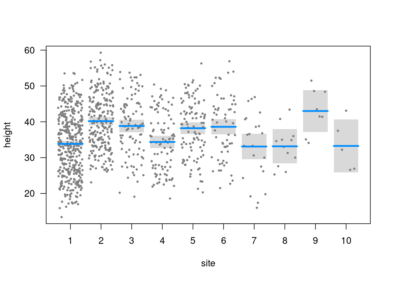

Plot (easystats)

plot(estimate_means(m3))

We selected `at = c("site")`.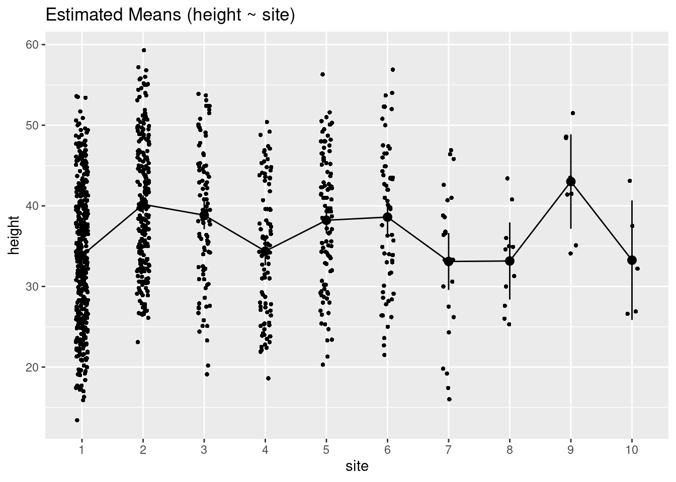

Plot model (modelsummary)

modelplot(m3)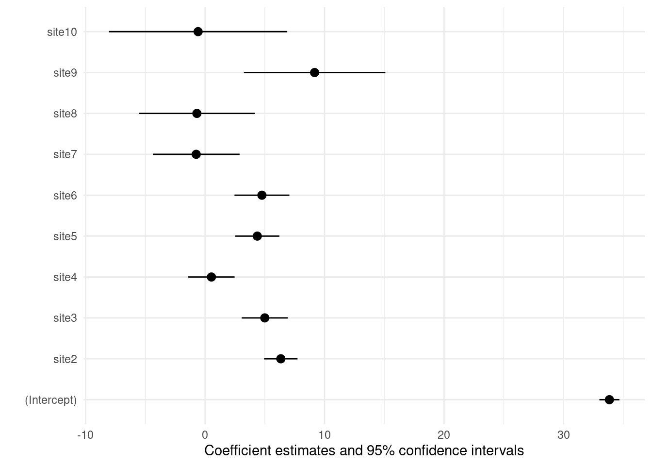

Plot model (easystats)

plot(parameters(m3), show_intercept = TRUE)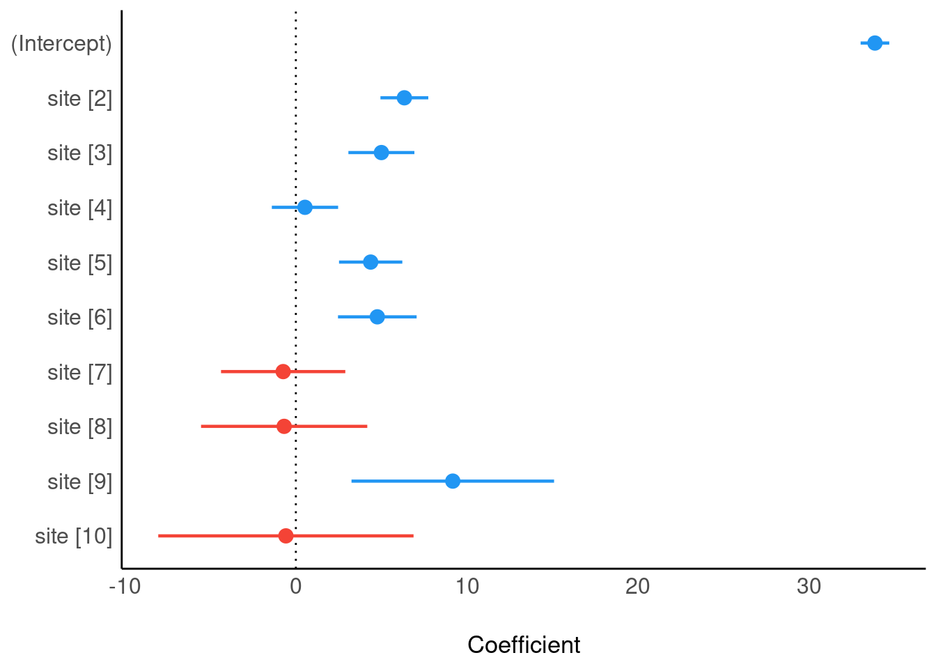

Fit model without intercept

m3bis <- lm(height ~ site - 1, data = trees)
summary(m3bis)

Call:
lm(formula = height ~ site - 1, data = trees)

Residuals:
     Min       1Q   Median       3Q      Max 
-20.4416  -6.9004   0.0379   6.3051  19.7584 

Coefficients:
       Estimate Std. Error t value Pr(>|t|)    
site1   33.8416     0.4266  79.329   <2e-16 ***
site2   40.1826     0.5707  70.404   <2e-16 ***
site3   38.8407     0.8854  43.868   <2e-16 ***
site4   34.3744     0.8903  38.610   <2e-16 ***
site5   38.2139     0.8404  45.469   <2e-16 ***
site6   38.6017     1.0904  35.401   <2e-16 ***
site7   33.1000     1.8007  18.381   <2e-16 ***
site8   33.1583     2.4382  13.599   <2e-16 ***
site9   43.0125     2.9862  14.404   <2e-16 ***
site10  33.2600     3.7773   8.805   <2e-16 ***
---
Signif. codes:  0 '***' 0.001 '**' 0.01 '*' 0.05 '.' 0.1 ' ' 1

Residual standard error: 8.446 on 990 degrees of freedom
Multiple R-squared:   0.95, Adjusted R-squared:  0.9495 
F-statistic:  1879 on 10 and 990 DF,  p-value: < 2.2e-16

plot(parameters(m3bis))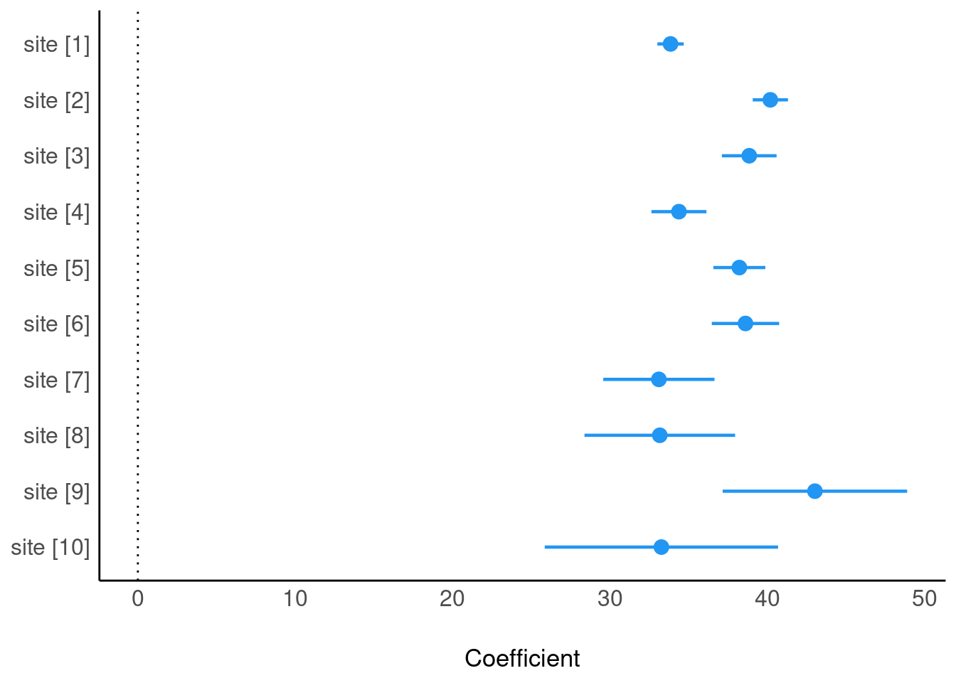

Model checking: residuals

def.par <- par(no.readonly = TRUE)
layout(matrix(1:4, nrow = 2))
plot(m3)

par(def.par)

Model checking: residuals

check_model(m3)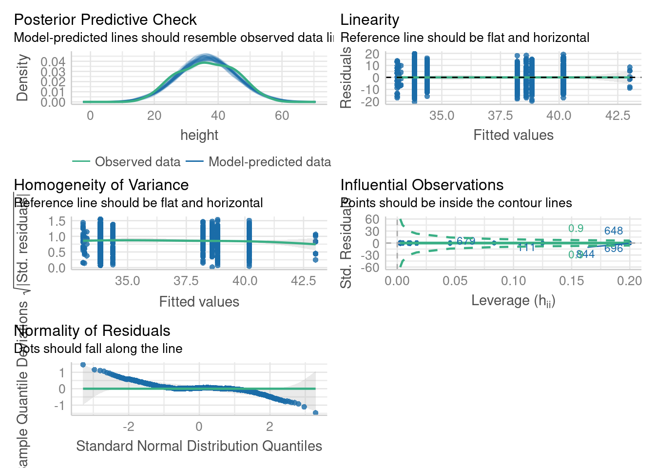

Combining continuous and categorical predictors

Predicting tree height based on dbh and site

lm(height ~ site + dbh, data = trees)

Call:
lm(formula = height ~ site + dbh, data = trees)

Coefficients:
(Intercept)        site2        site3        site4        site5        site6  
    16.6990       6.5043       4.3575       1.9347       3.6374       4.2045  
      site7        site8        site9       site10          dbh  
    -0.1762      -5.3126       5.4370       2.2633       0.6171  

corresponds to

\[ \begin{aligned} y_{i} = a + b_{site2} + c_{site3} + d_{site4} + e_{site5} +...+ k \cdot DBH_{i} + \varepsilon _{i} \\ \varepsilon _{i}\sim N\left( 0,\sigma^2 \right) \\ \end{aligned} \]

Predicting tree height based on dbh and site

m4 <- lm(height ~ site + dbh, data = trees)
summary(m4)

Call:
lm(formula = height ~ site + dbh, data = trees)

Residuals:
     Min       1Q   Median       3Q      Max 
-10.1130  -1.9885   0.0582   2.0314  11.3320 

Coefficients:
             Estimate Std. Error t value Pr(>|t|)    
(Intercept) 16.699037   0.260565  64.088  < 2e-16 ***
site2        6.504303   0.256730  25.335  < 2e-16 ***
site3        4.357457   0.354181  12.303  < 2e-16 ***
site4        1.934650   0.356102   5.433 6.98e-08 ***
site5        3.637432   0.339688  10.708  < 2e-16 ***
site6        4.204511   0.421906   9.966  < 2e-16 ***
site7       -0.176193   0.666772  -0.264   0.7916    
site8       -5.312648   0.893603  -5.945 3.82e-09 ***
site9        5.437049   1.087766   4.998 6.84e-07 ***
site10       2.263338   1.369986   1.652   0.0988 .  
dbh          0.617075   0.007574  81.473  < 2e-16 ***
---
Signif. codes:  0 '***' 0.001 '**' 0.01 '*' 0.05 '.' 0.1 ' ' 1

Residual standard error: 3.043 on 989 degrees of freedom
Multiple R-squared:  0.8835,    Adjusted R-squared:  0.8823 
F-statistic:   750 on 10 and 989 DF,  p-value: < 2.2e-16

Presenting model results

parameters(m4)

Parameter   | Coefficient |       SE |         95% CI | t(989) |      p
-----------------------------------------------------------------------
(Intercept) |       16.70 |     0.26 | [16.19, 17.21] |  64.09 | < .001
site [2]    |        6.50 |     0.26 | [ 6.00,  7.01] |  25.34 | < .001
site [3]    |        4.36 |     0.35 | [ 3.66,  5.05] |  12.30 | < .001
site [4]    |        1.93 |     0.36 | [ 1.24,  2.63] |   5.43 | < .001
site [5]    |        3.64 |     0.34 | [ 2.97,  4.30] |  10.71 | < .001
site [6]    |        4.20 |     0.42 | [ 3.38,  5.03] |   9.97 | < .001
site [7]    |       -0.18 |     0.67 | [-1.48,  1.13] |  -0.26 | 0.792 
site [8]    |       -5.31 |     0.89 | [-7.07, -3.56] |  -5.95 | < .001
site [9]    |        5.44 |     1.09 | [ 3.30,  7.57] |   5.00 | < .001
site [10]   |        2.26 |     1.37 | [-0.43,  4.95] |   1.65 | 0.099 
dbh         |        0.62 | 7.57e-03 | [ 0.60,  0.63] |  81.47 | < .001

Uncertainty intervals (equal-tailed) and p-values (two-tailed) computed
  using a Wald t-distribution approximation.

Estimated tree heights for each site

estimate_means(m4)

We selected `at = c("site")`.

Estimated Marginal Means

site |  Mean |   SE |         95% CI
------------------------------------
1    | 33.90 | 0.15 | [33.60, 34.21]
2    | 40.41 | 0.21 | [40.01, 40.81]
3    | 38.26 | 0.32 | [37.64, 38.89]
4    | 35.84 | 0.32 | [35.21, 36.47]
5    | 37.54 | 0.30 | [36.95, 38.14]
6    | 38.11 | 0.39 | [37.34, 38.88]
7    | 33.73 | 0.65 | [32.45, 35.00]
8    | 28.59 | 0.88 | [26.86, 30.32]
9    | 39.34 | 1.08 | [37.23, 41.45]
10   | 36.17 | 1.36 | [33.50, 38.84]

Marginal means estimated at site

Fit model without intercept

m4 <- lm(height ~ -1 + site + dbh, data = trees)
summary(m4)

Call:
lm(formula = height ~ -1 + site + dbh, data = trees)

Residuals:
     Min       1Q   Median       3Q      Max 
-10.1130  -1.9885   0.0582   2.0314  11.3320 

Coefficients:
        Estimate Std. Error t value Pr(>|t|)    
site1  16.699037   0.260565   64.09   <2e-16 ***
site2  23.203340   0.292773   79.25   <2e-16 ***
site3  21.056494   0.386532   54.48   <2e-16 ***
site4  18.633687   0.374456   49.76   <2e-16 ***
site5  20.336469   0.373942   54.38   <2e-16 ***
site6  20.903548   0.448913   46.56   <2e-16 ***
site7  16.522844   0.679936   24.30   <2e-16 ***
site8  11.386389   0.918198   12.40   <2e-16 ***
site9  22.136086   1.105970   20.02   <2e-16 ***
site10 18.962375   1.372158   13.82   <2e-16 ***
dbh     0.617075   0.007574   81.47   <2e-16 ***
---
Signif. codes:  0 '***' 0.001 '**' 0.01 '*' 0.05 '.' 0.1 ' ' 1

Residual standard error: 3.043 on 989 degrees of freedom
Multiple R-squared:  0.9935,    Adjusted R-squared:  0.9934 
F-statistic: 1.377e+04 on 11 and 989 DF,  p-value: < 2.2e-16

Plot (visreg)

visreg(m4)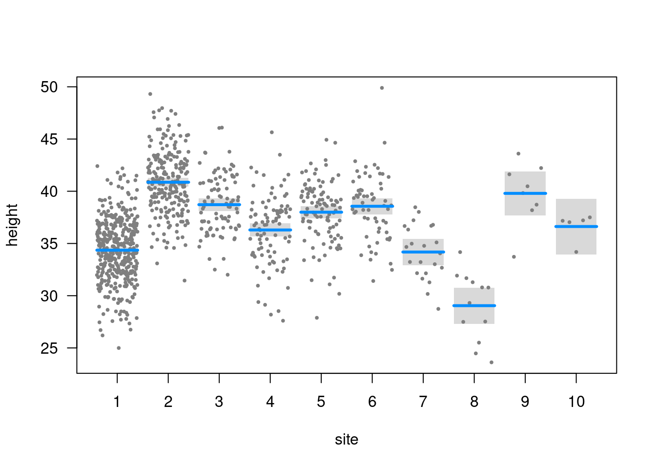

visreg(m4, xvar = "dbh", by = "site", overlay = TRUE, band = FALSE)

Plot model (easystats)

plot(parameters(m4))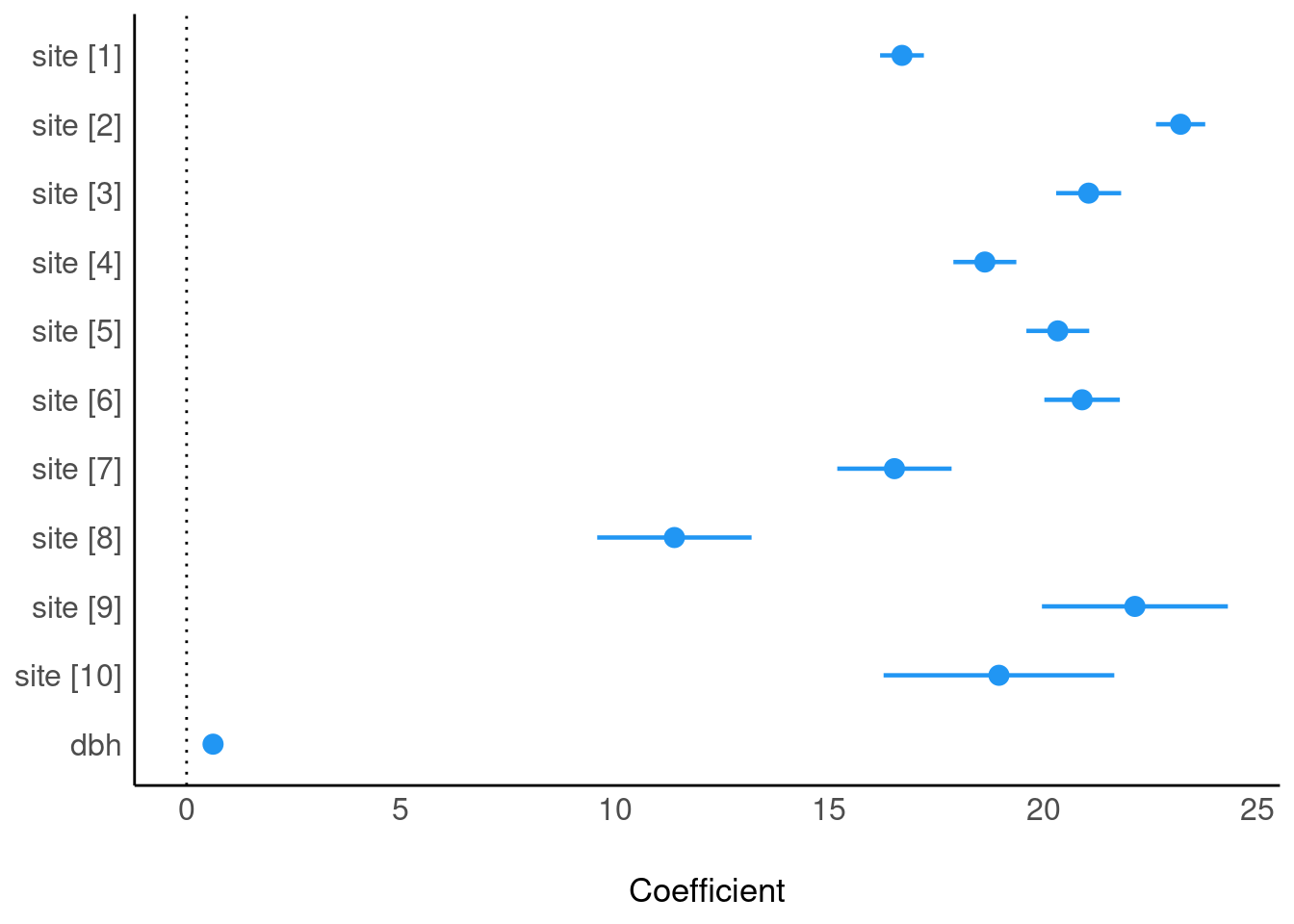

Keeping sites only, dropping “dbh”

plot(parameters(m4, drop = "dbh"))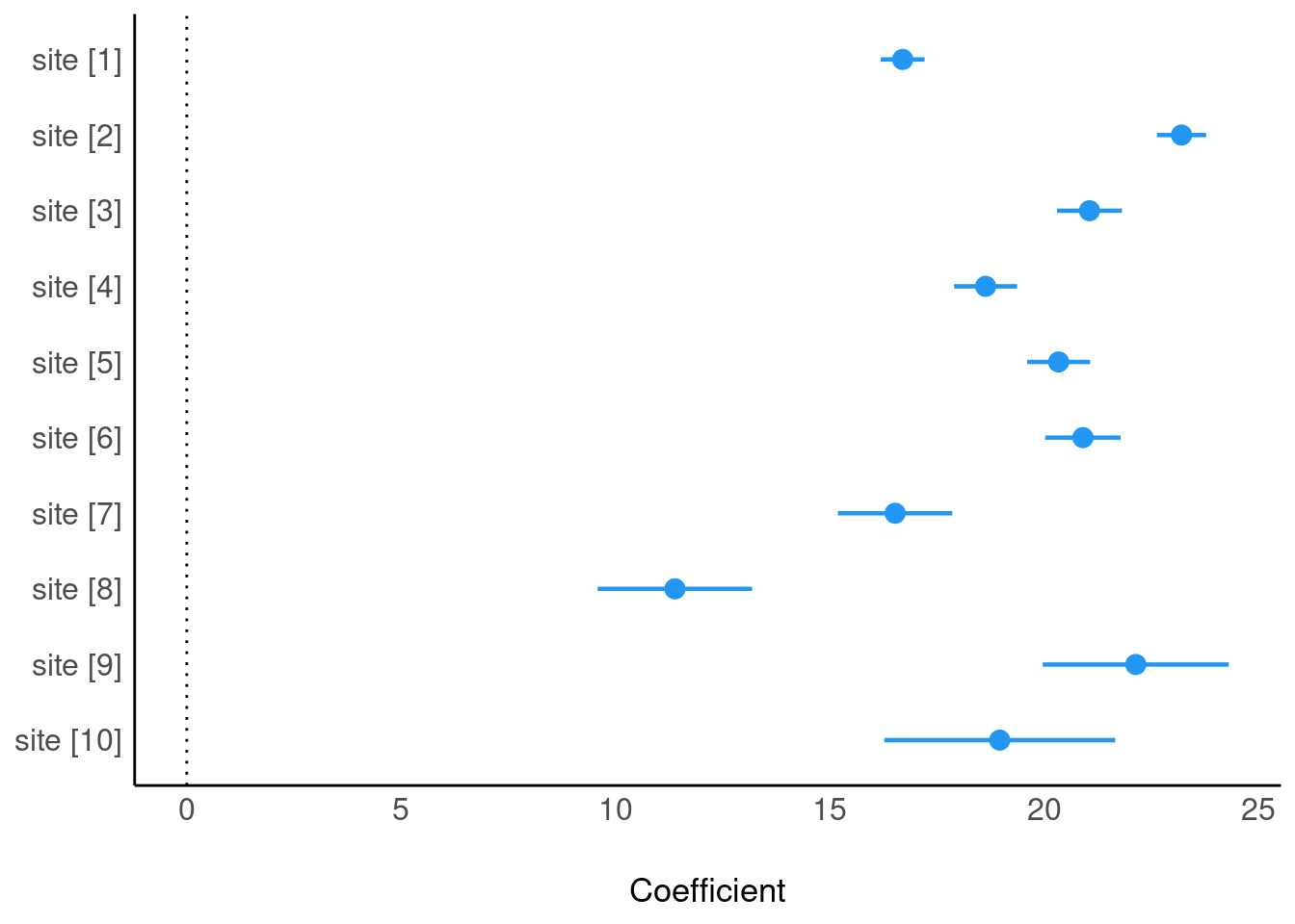

Plot model (modelsummary)

modelplot(m4)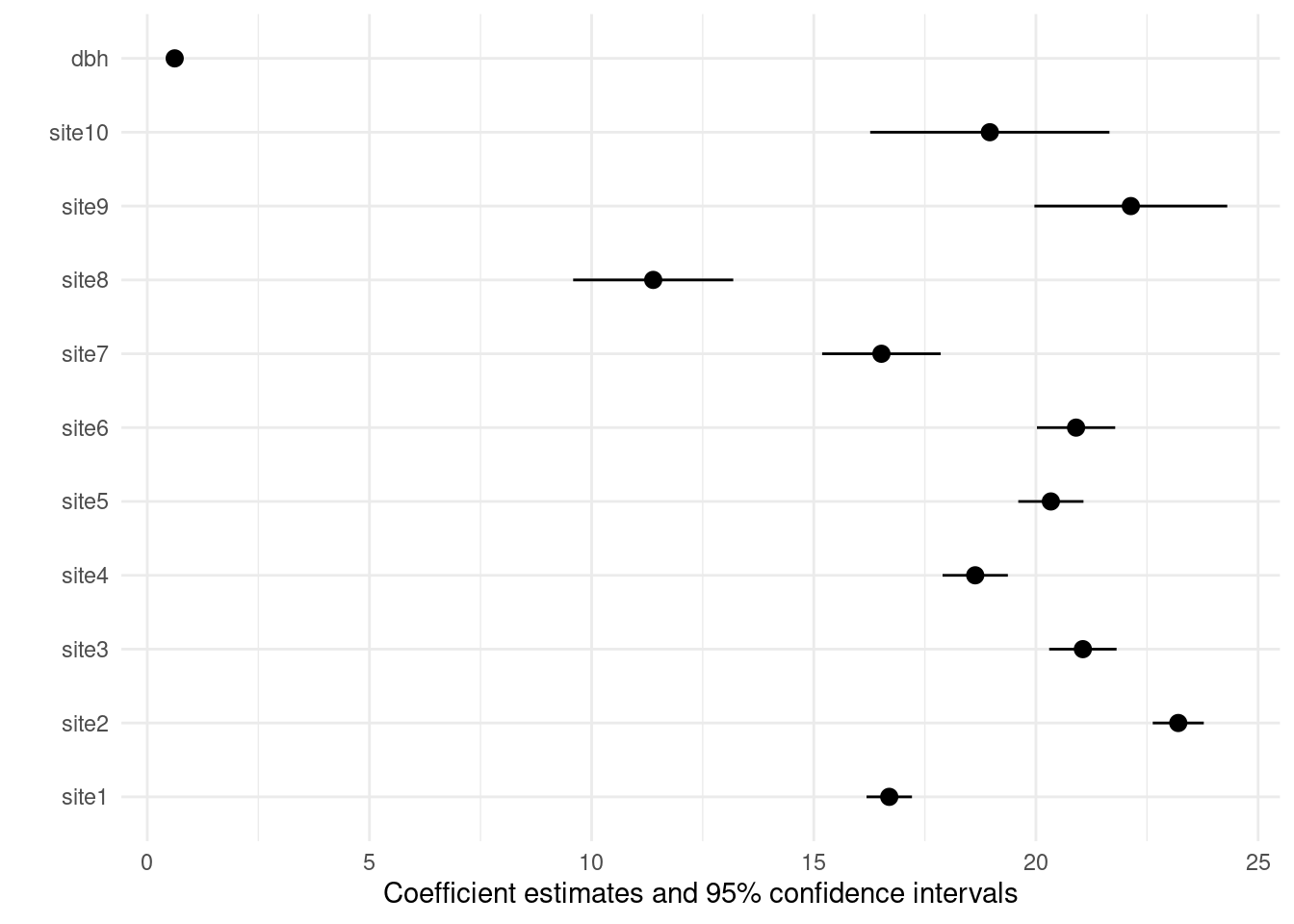

Keeping sites only, dropping “dbh”

modelplot(m4, coef_omit = "dbh")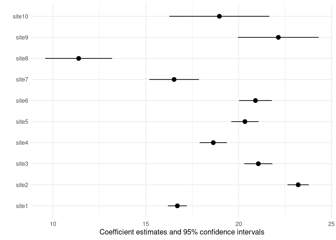

What happened to site 8?

visreg(m3)

visreg(m4, xvar = "site")

site 8 has the largest diameters:

boxplot(dbh ~ site, data = trees)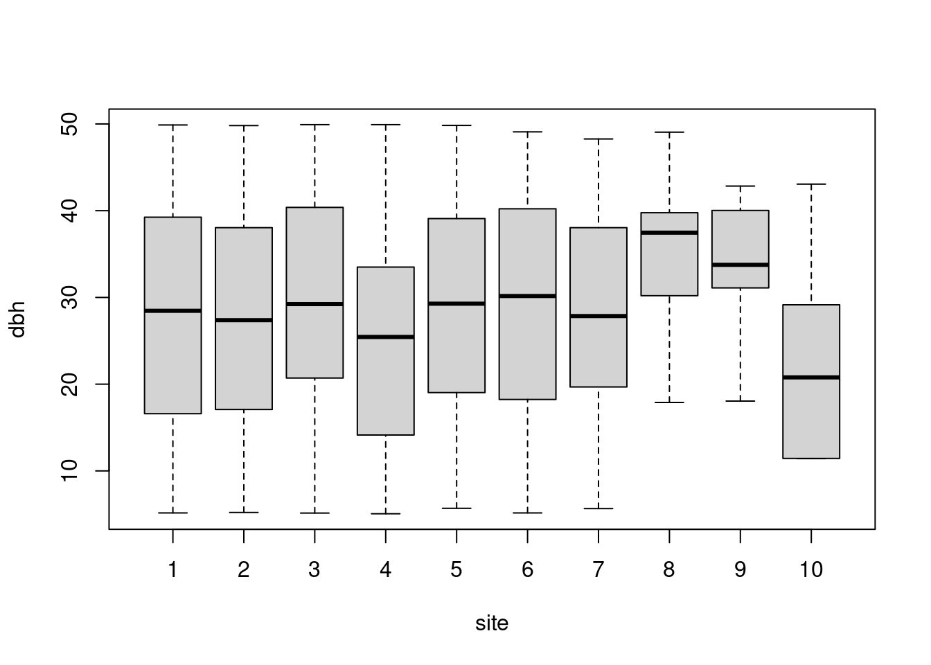

DBH

aggregate(trees$dbh ~ trees$site, FUN = mean)

   trees$site trees$dbh
1           1  27.78033
2           2  27.51580
3           3  28.82011
4           4  25.50867
5           5  28.97119
6           6  28.68067
7           7  26.86409
8           8  35.28250
9           9  33.83125
10         10  23.17000

HEIGHT

aggregate(trees$height ~ trees$site, FUN = mean)

   trees$site trees$height
1           1     33.84158
2           2     40.18265
3           3     38.84066
4           4     34.37444
5           5     38.21386
6           6     38.60167
7           7     33.10000
8           8     33.15833
9           9     43.01250
10         10     33.26000

We have fitted model w/ many intercepts and single slope

visreg(m4, xvar = "dbh", by = "site", overlay = TRUE, band = FALSE)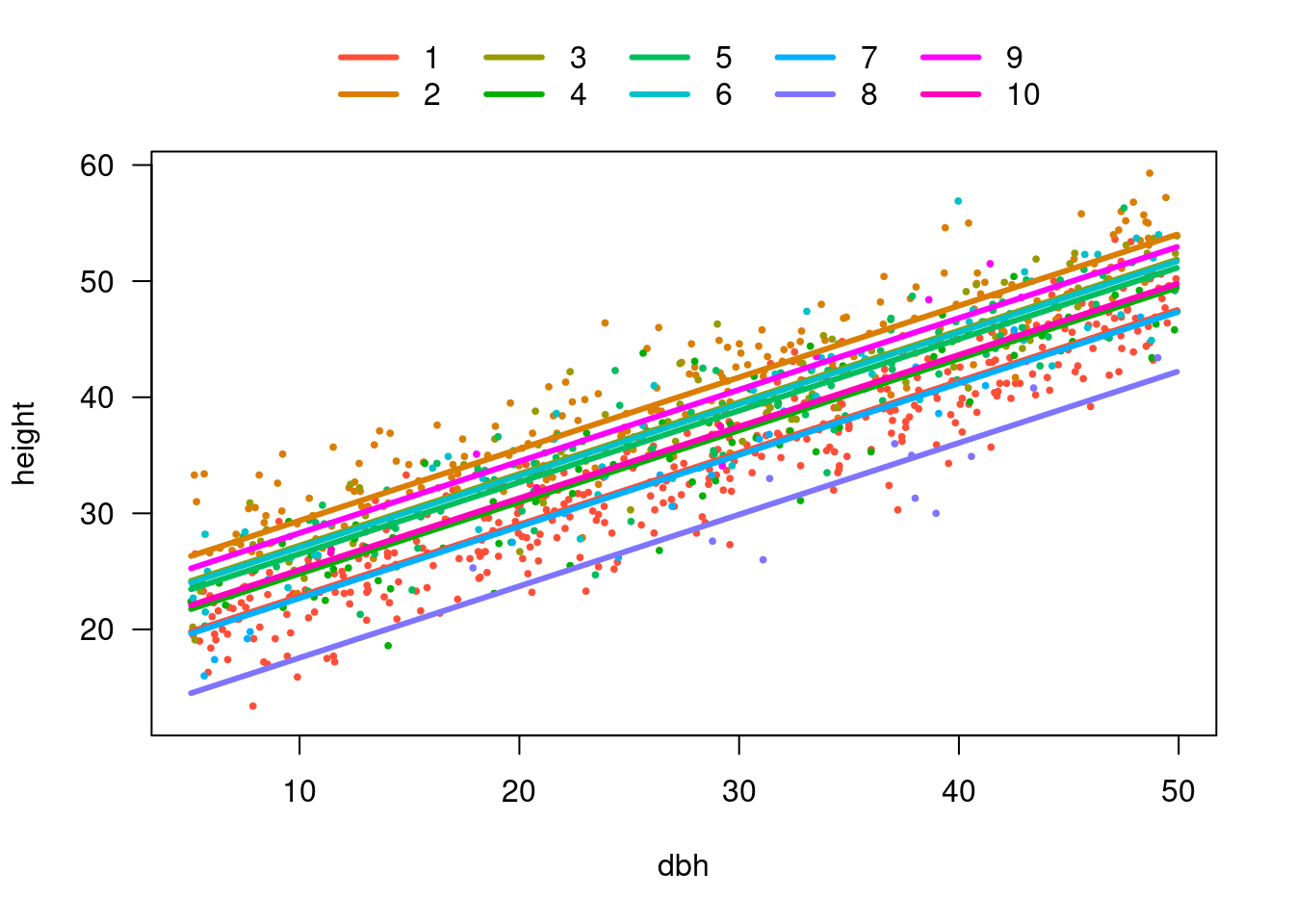

Slope is the same for all sites

parameters(m4, keep = "dbh")

Parameter | Coefficient |       SE |       95% CI | t(989) |      p
-------------------------------------------------------------------
dbh       |        0.62 | 7.57e-03 | [0.60, 0.63] |  81.47 | < .001

Uncertainty intervals (equal-tailed) and p-values (two-tailed) computed
  using a Wald t-distribution approximation.

Model checking: residuals

def.par <- par(no.readonly = TRUE)
layout(matrix(1:4, nrow=2))
plot(m4)

par(def.par)

Model checking with easystats

check_model(m4)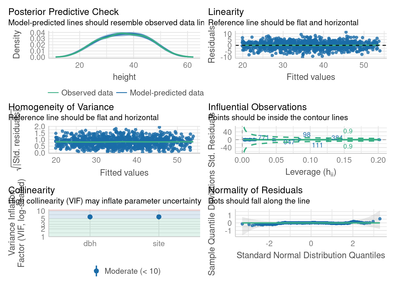

How good is this model? Calibration plot

trees$height.pred <- fitted(m4)
plot(trees$height.pred, trees$height, 
     xlab = "Tree height (predicted)", 
     ylab = "Tree height (observed)", 
     las = 1, xlim = c(10,60), ylim = c(10,60))
abline(a = 0, b = 1)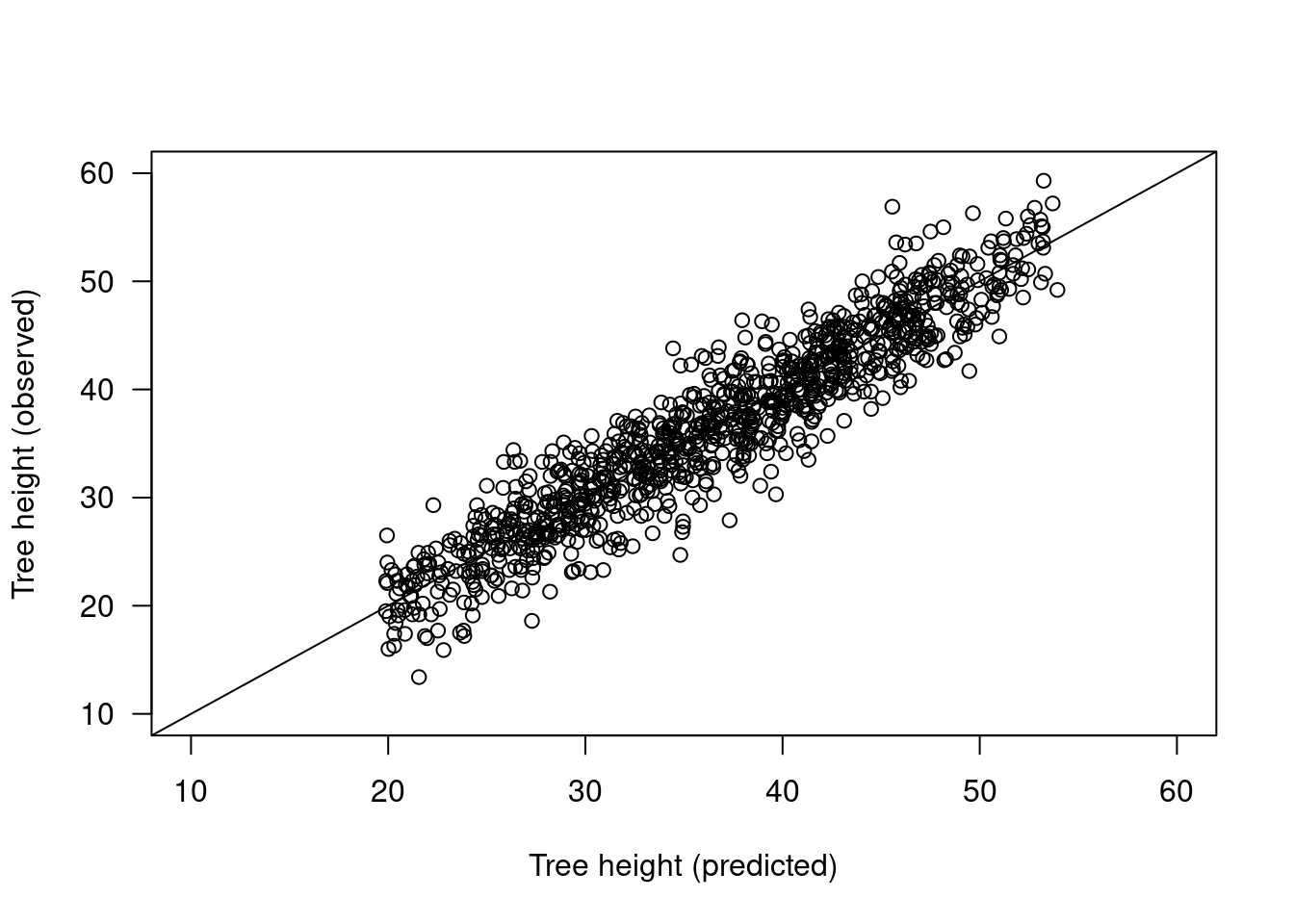

How good is this model? Calibration plot (easystats)

pred <- estimate_expectation(m4)
pred$obs <- trees$height
plot(obs ~ Predicted, data = pred, xlim = c(15, 60), ylim = c(15, 60))
abline(a = 0, b = 1)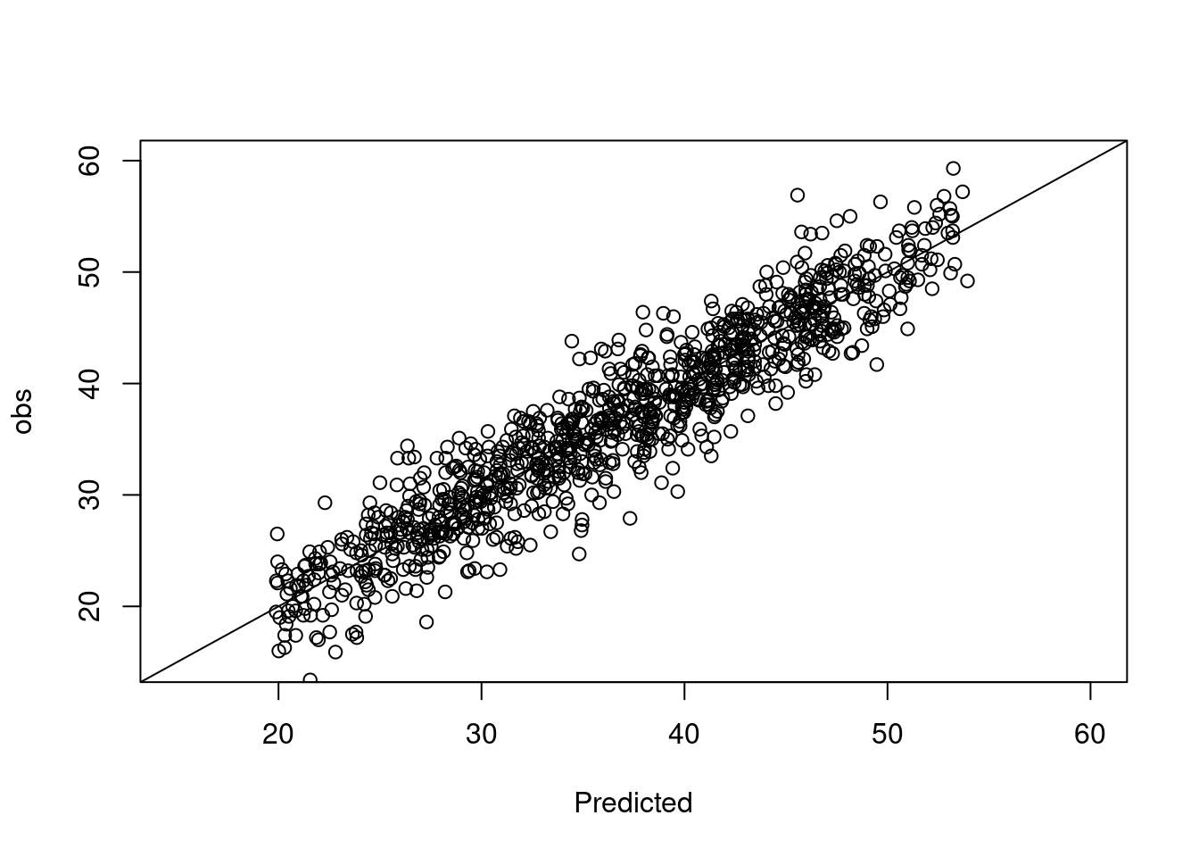

Posterior predictive checking

Simulating response data from fitted model (yrep)

and comparing with observed response (y)

check_predictions(m4)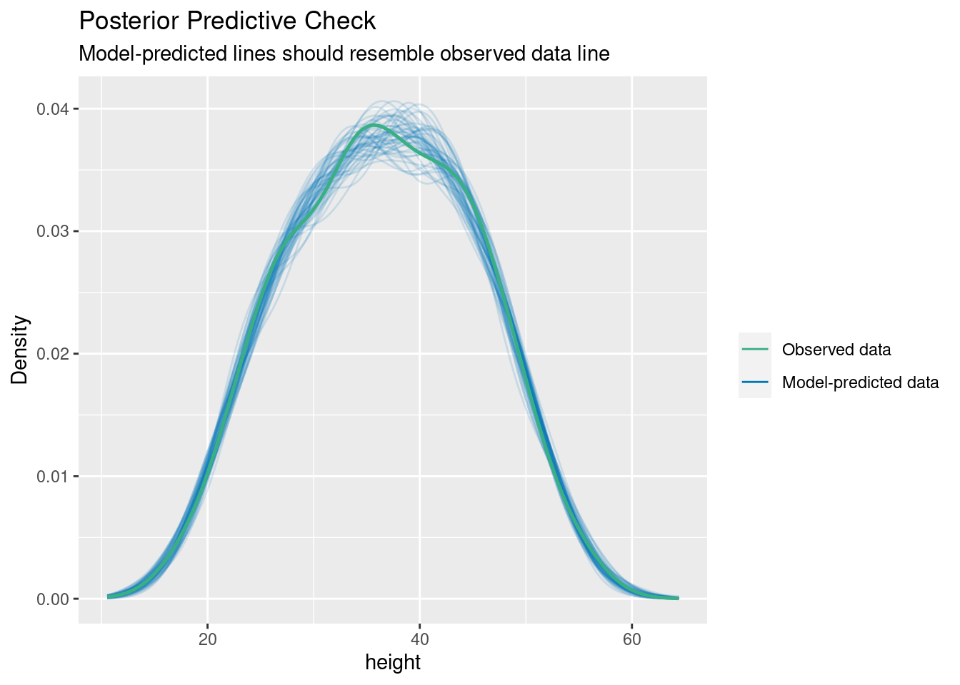

Predicting heights of new trees (easystats)

Using model for prediction

Expected height of 10-cm diameter tree in each site?

trees.10cm <- data.frame(site = as.factor(1:10),
                        dbh = 10)
trees.10cm

   site dbh
1     1  10
2     2  10
3     3  10
4     4  10
5     5  10
6     6  10
7     7  10
8     8  10
9     9  10
10   10  10

Using model for prediction

Expected height of 10-cm DBH trees at each site

pred <- estimate_expectation(m4, data = trees.10cm)
pred

Model-based Expectation

site |   dbh | Predicted |   SE |         95% CI
------------------------------------------------
1    | 10.00 |     22.87 | 0.20 | [22.47, 23.27]
2    | 10.00 |     29.37 | 0.24 | [28.89, 29.85]
3    | 10.00 |     27.23 | 0.35 | [26.54, 27.91]
4    | 10.00 |     24.80 | 0.34 | [24.13, 25.47]
5    | 10.00 |     26.51 | 0.34 | [25.85, 27.16]
6    | 10.00 |     27.07 | 0.42 | [26.25, 27.89]
7    | 10.00 |     22.69 | 0.66 | [21.40, 23.99]
8    | 10.00 |     17.56 | 0.90 | [15.79, 19.32]
9    | 10.00 |     28.31 | 1.09 | [26.17, 30.45]
10   | 10.00 |     25.13 | 1.36 | [22.46, 27.81]

Variable predicted: height

Using model for prediction

Prediction intervals (accounting for residual variance)

pred <- estimate_prediction(m4, data = trees.10cm)
pred

Model-based Prediction

site |   dbh | Predicted |   SE |         95% CI
------------------------------------------------
1    | 10.00 |     22.87 | 3.05 | [16.88, 28.85]
2    | 10.00 |     29.37 | 3.05 | [23.38, 35.36]
3    | 10.00 |     27.23 | 3.06 | [21.22, 33.24]
4    | 10.00 |     24.80 | 3.06 | [18.80, 30.81]
5    | 10.00 |     26.51 | 3.06 | [20.50, 32.51]
6    | 10.00 |     27.07 | 3.07 | [21.05, 33.10]
7    | 10.00 |     22.69 | 3.11 | [16.58, 28.80]
8    | 10.00 |     17.56 | 3.17 | [11.33, 23.78]
9    | 10.00 |     28.31 | 3.23 | [21.96, 34.65]
10   | 10.00 |     25.13 | 3.33 | [18.59, 31.68]

Variable predicted: height

Q: Does allometric relationship between Height and Diameter vary among sites?

df <- data.frame(dbh = seq(10, 50, by = 1), 
                 height = seq(20, 60, by = 1))

plot(height ~ dbh, data = df, type = "n")
abline(a = 25, 0.6)
abline(a = 40, b = 0.1, col = "steelblue")
abline(a = 50, b = -0.3, col = "orangered")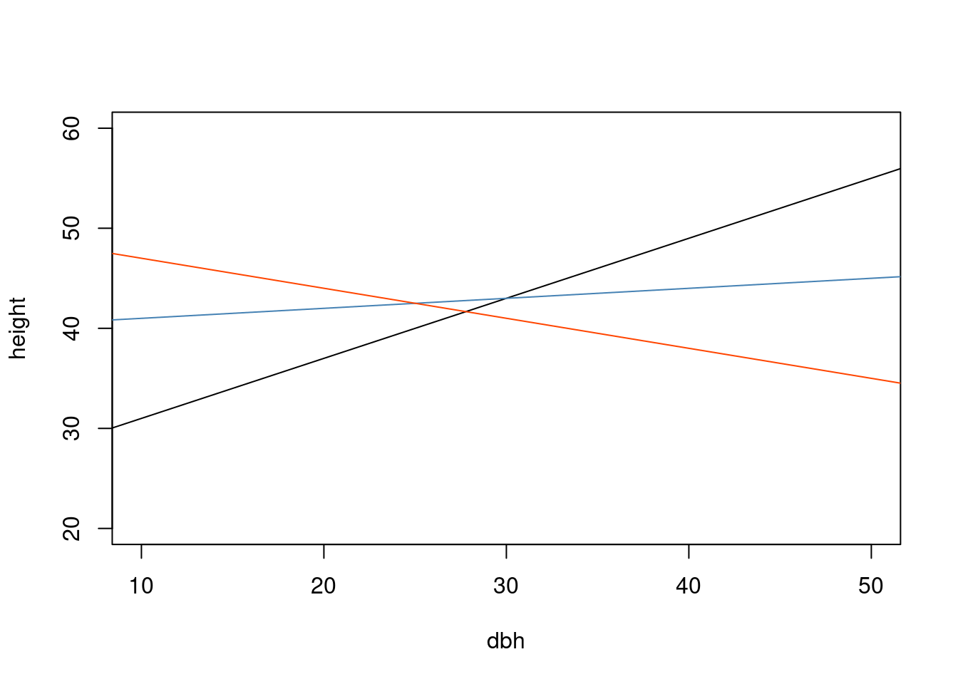

Model with interactions

m5 <- lm(height ~ site*dbh, data = trees)
summary(m5)

Call:
lm(formula = height ~ site * dbh, data = trees)

Residuals:
     Min       1Q   Median       3Q      Max 
-10.1017  -1.9839   0.0645   2.0486  11.1789 

Coefficients:
             Estimate Std. Error t value Pr(>|t|)    
(Intercept) 16.359437   0.360054  45.436  < 2e-16 ***
site2        7.684781   0.609657  12.605  < 2e-16 ***
site3        4.518568   0.867008   5.212 2.28e-07 ***
site4        2.769336   0.813259   3.405 0.000688 ***
site5        3.917607   0.870983   4.498 7.68e-06 ***
site6        4.155161   1.009379   4.117 4.17e-05 ***
site7       -2.306799   1.551303  -1.487 0.137334    
site8       -2.616095   4.090671  -0.640 0.522630    
site9        2.621560   5.073794   0.517 0.605492    
site10       4.662340   2.991072   1.559 0.119378    
dbh          0.629299   0.011722  53.685  < 2e-16 ***
site2:dbh   -0.042784   0.020033  -2.136 0.032950 *  
site3:dbh   -0.006031   0.027640  -0.218 0.827312    
site4:dbh   -0.031633   0.028225  -1.121 0.262677    
site5:dbh   -0.010173   0.027887  -0.365 0.715334    
site6:dbh    0.001337   0.032109   0.042 0.966797    
site7:dbh    0.079728   0.052056   1.532 0.125951    
site8:dbh   -0.079027   0.113386  -0.697 0.485984    
site9:dbh    0.081035   0.146649   0.553 0.580679    
site10:dbh  -0.101107   0.114520  -0.883 0.377522    
---
Signif. codes:  0 '***' 0.001 '**' 0.01 '*' 0.05 '.' 0.1 ' ' 1

Residual standard error: 3.041 on 980 degrees of freedom
Multiple R-squared:  0.8847,    Adjusted R-squared:  0.8825 
F-statistic: 395.7 on 19 and 980 DF,  p-value: < 2.2e-16

Does slope vary among sites?

visreg(m5, xvar = "dbh", by = "site")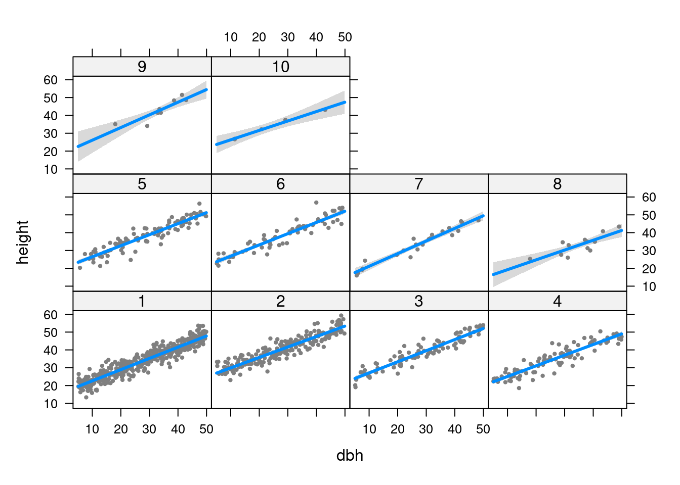

visreg(m5, xvar = "dbh", by = "site", overlay = TRUE, band = FALSE)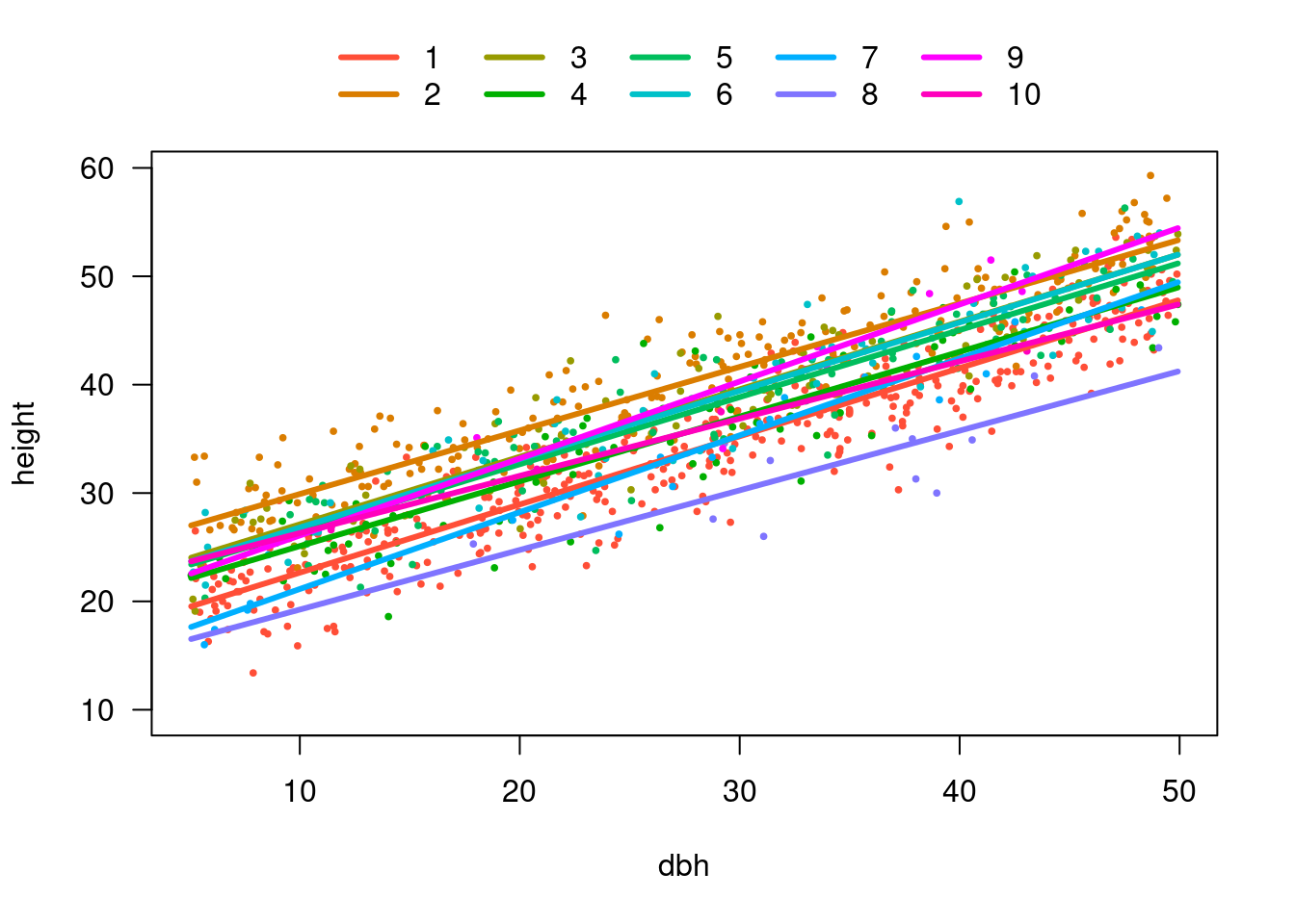

END