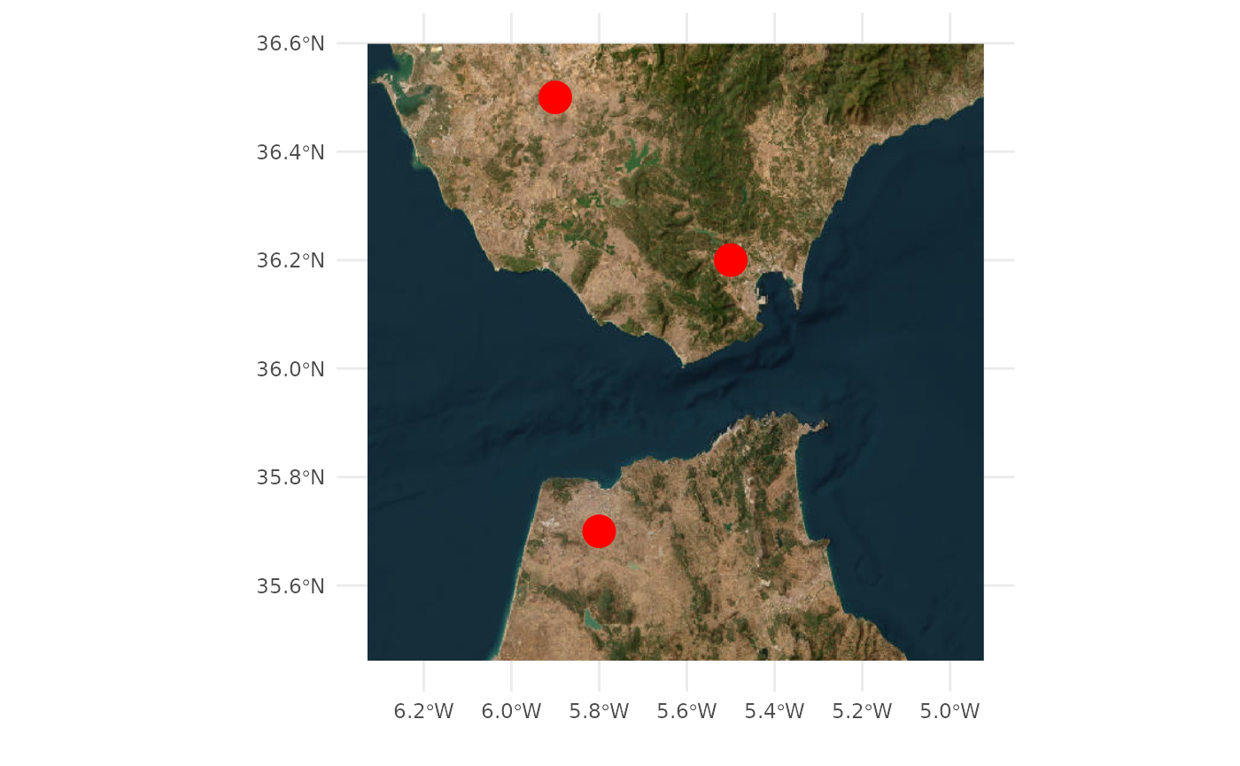
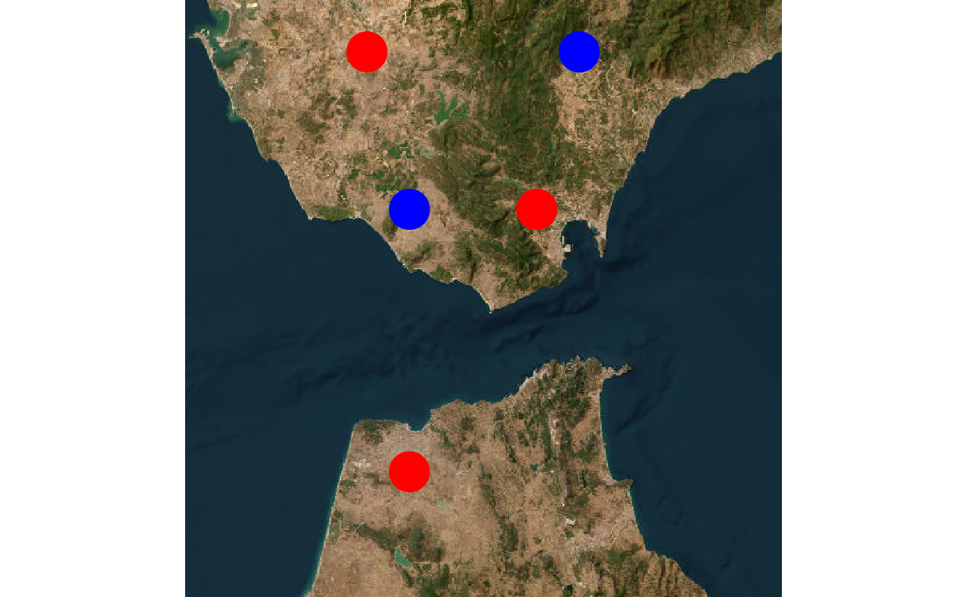
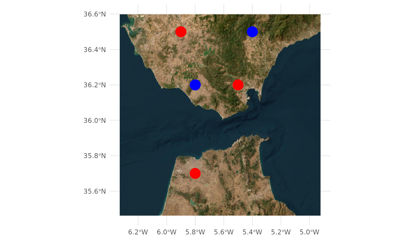
Map occurrences (point coordinates) • rSDM

library(rSDM)

Let’s create example point coordinates and convert them to a spatial (sf) object:

locs <- data.frame(lon = c(-5.8, -5.5, -5.9), lat = c(35.7, 36.2, 36.5))
locs <- locs2sf(locs, crs = 4326)
locs
#> Simple feature collection with 3 features and 0 fields
#> Geometry type: POINT
#> Dimension:     XY
#> Bounding box:  xmin: -5.9 ymin: 35.7 xmax: -5.5 ymax: 36.5
#> Geodetic CRS:  WGS 84
#>            geometry
#> 1 POINT (-5.8 35.7)
#> 2 POINT (-5.5 36.2)
#> 3 POINT (-5.9 36.5)

Note that SpatVector objects (from terra) are also accepted, and can be created using rSDM::locs2vect().

Default map with occmap

Unless a raster ras is provided, occmap will automatically download a background map from the internet.

occmap(locs, psize = 6)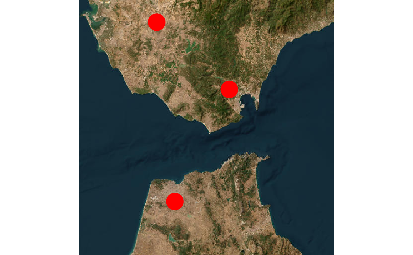

The background map can be easily changed using the bg argument:

occmap(locs, psize = 6, bg = "CartoDB.Positron")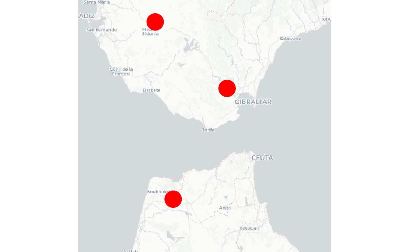

Interactive (leaflet) map

occmap(locs, psize = 6, type = "leaflet")

occmap(locs, psize = 6, type = "leaflet", bg = "CartoDB.Positron")

ggplot map

occmap(locs, psize = 6, type = "ggplot")

Adding points to a previous map

Let’s create some new coordinates (e.g. for a different species):

new.locs <- data.frame(lon = c(-5.8, -5.4), lat = c(36.2, 36.5))
new.locs.sf <- locs2sf(new.locs, crs = 4326)

Using ‘base’ maps

Note the add = TRUE argument:

map <- occmap(locs, psize = 6)
occmap(new.locs.sf, add = TRUE, psize = 6, pcol = "blue")

Adding points to a previous map (leaflet)

Note the previous map has to be provided (using prev.map argument):

map <- occmap(locs, psize = 6, type = "leaflet")
occmap(new.locs.sf, prev.map = map, psize = 6, pcol = "blue")

Adding points to a previous map (ggplot)

Note the previous map has to be provided (using prev.map argument):

map <- occmap(locs, psize = 6, type = "ggplot")
occmap(new.locs.sf, prev.map = map, psize = 6, pcol = "blue")